1
Ichthyoplankton and Fish post-larvae
Survey
This Annex presents the methodology,
results and conclusions of a nine month Ichthyoplankton
and Fish Post-Larvae Survey (the Survey) aimed at assessing the
abundance, composition and spatial distribution of fish within a previously
identified spawning and nursing area in the southern waters of
The ultimate objective of the present
survey is to determine how the abundance and diversity of ichthyoplankton and
fish post-larvae differs between various sites within the southern waters. The information has then been fed into the
fisheries impact assessment for the South Soko LNG terminal.
Of most interest to the Survey is the relative abundance and
diversity of fish fry, larvae and eggs at different locations within the
spawning and nursery ground in the southern waters of
A total of 20 sampling locations were
identified (Table 1.1 and Figure
1.1).
These stations were selected to represent habitat type or topography
(e.g., sandy bay, rocky reef or open channel).
Table 1.1 Sampling Locations
|
Survey Area |
Number of Stations |
Stations ID |
|
North and |
5 |
SK1 – SK5 |
|
|
6 |
FL1, FL2, PH1, PH2, YO1, YO2 |
|
|
3 |
AC1, SL1, TF1 |
|
South Cheung Chau and Shek Kwu Chau |
3 |
SKC1, SKC2, CC1 |
|
|
3 |
L1, L2, SW1 |
The Survey
assesses the relative abundance and diversity of fish fry and larvae using two
survey methods:
1.
Ichthyoplankton Sampling: The
first method was an ichthyoplankton survey to determine the abundance and
species composition of fish larval assemblages.
During this stage, fish are still in their planktonic phase and drift
with the water currents,
2.
Fish post Larvae Sampling: The
second method was a fish post-larval or juvenile survey to determine the
abundance and species composition of post-settlement stages. At this stage fish have attained a larger
size and are no longer planktonic, thus are capable of swimming against currents
or have adopted a largely demersal habit.
Ichthyoplankton and fish post-larvae
surveys were conducted twice per month for nine months from July 2005 to March
2006 at each of the 20 sampling locations (Table
1.2). The surveys were designed to
assess the abundance and composition of ichthyoplankton and fish post-larvae
throughout the water column and covered both the wet (July to October) and dry
(November to March) seasons in order to account for any seasonal variations in
abundance and diversity. Samples were
collected during day-time (7am – 7pm) by towing with plankton nets across the
entire water column (Section 1.2.3).
In addition, discrete depth surveys
(surface/near-bottom) were conducted on a diurnal/nocturnal basis at stations
SK1 and SK2 in July and August 2005 and at SK3, SK4, SK5, SW1, L1 and L2 in
August 2005 (Table 1.2).
SK1 and SK2 were chosen for additional
sampling as they represent the broad location of the proposed intake of the
open circuit vaporisation system, whilst SK3, SK4, SK5, SW1, L1 and L2 were
chosen as reference locations. Discrete
depth sampling was completed in order to determine the vertical distribution of
fish fry and ichthyoplankton, whilst diurnal/nocturnal sampling allowed to determine
any day/night vertical migration of the fish larvae and post-larvae.
The results from the surface/bottom and
day/night surveys were then fed into the impact assessment to better identify
the potential impacts associated with the open circuit vaporization system of
the proposed LNG terminal.
Table 1.1 Sampling Schedule During
July 2005 to March 2006
|
Month |
Entire Water Column Sampling |
Discrete Depths Samples(1) |
||||
|
Ichthyo-plankton |
Fish post larvae |
Date |
Ichthyo-plankton |
Fish post larvae |
Date |
|
|
Jul 2005 |
2 |
2 |
23,
24, 25, 28, 29, 30 |
1 |
1 |
25
and 29 |
|
Aug 2005 |
2 |
2 |
10,
15, 16, 24, 25, 26, 29, 30 |
1 |
1 |
16,
24, 26, 27, 29, 30 |
|
Sep 2005 |
2 |
2 |
9,
12, 13, 27, 28, 29 |
0 |
0 |
N/A |
|
Oct 2005 |
2 |
2 |
12, 13, 21, 24, 25, 26 |
0 |
0 |
N/A |
|
Nov 2005 |
2 |
2 |
8, 9, 11, 21, 22, 23, 24 |
0 |
0 |
N/A |
|
Dec 2005 |
2 |
2 |
5,
6, 7, 20, 21, 23 |
0 |
0 |
N/A |
|
Jan 2006 |
2 |
2 |
4,
5, 6, 23, 24, 25 |
0 |
0 |
N/A |
|
Feb 2006 |
2 |
2 |
1,
2, 3, 6, 7, 8 |
0 |
0 |
N/A |
|
Mar 2006 |
2 |
2 |
15,
16, 17, 20, 21, 22 |
0 |
0 |
N/A |
|
(1) Diurnal and Nocturnal
Samples (2) n/a
surveys were conducted during the summer months to represent the peak periods
of fish eggs and larval abundance |
||||||
1.2.2
Field Survey Equipment
The
field equipment used in the Survey is
presented in Table 1.3.
Table 1.2 Equipment list of the Ichthyoplankton
and Fish Post-Larvae Surveys
|
Instrument |
Manufacturer and Model number |
|
Bongo Ring net |
Aquatic research Instruments, 50cm
mouth diameter, mesh size 0.3 mm |
|
|
Aquatic research Instruments, 50cm
mouth diameter, mesh size 0.5 mm |
|
Closing Plankton net |
Aquatic research Instruments, 50cm
mouth diameter, mesh size 0.3 mm |
|
|
Aquatic research Instruments, 50cm
mouth diameter, mesh size 0.5 mm |
|
CTD |
SBE 25 Sealogger CTD |
|
Flowmeter |
General Oceanics Inc. Model 2030R |
|
|
G.O. Environmental Model |
|
Sample containers |
Nalgene Jar Straight-side 2118-0016
500mL |
|
|
Naglene Jar Straight-side 2118-0032
1000mL |
The quantity of fish larvae and
post-larvae collected from each of the samples were calculated in terms of
number per volume of water filtered during the tow, i.e. standardized as number
of fish per 100m3 of water filtered.
This in effect provided a measure of fish density per sample, thus
allowing direct comparisons between samples.
Flowmeters were fitted to the mouths of
the nets to record the actual amount of water flowing through the nets during
towing, from which the volume filtered was derived.
A Conductivity-Temperature-Depth (CTD)
recorder was also deployed at each sampling station to obtain a vertical
profile of physical environmental parameters with depth, including temperature,
salinity, dissolved oxygen, turbidity, and chlorophyll-a concentration (as a
measure of phytoplankton abundance).
The depth and seabed topography was
determined at each station using an on board echo-sounder.
1.2.3
Sampling Methodologies
Ichthyoplankton
A plankton net, typically of 50 cm mouth
diameter and with 0.3 mm mesh size, was deployed to collect zooplankton and
ichthyoplankton. A flowmeter was fitted
at the mouth of the net to record the volume of water filtered. Before each towing, the CTD was deployed to
obtain vertical profile of physical environmental parameters.
The plankton material was fixed in 4%
formalin buffered with seawater immediately after collection onboard, and then
transferred into 70% ethanol for subsequent preservation in the laboratory.
The ichthyoplankton samples were sorted in
the laboratory, where all fish larvae were sorted and counted. Identifications of fish larvae were made
under dissecting stereomicroscopes to the appropriate taxon using available
identification keys. Fish larvae were
measured following conventional methodology (total lengths and standard
lengths) to determine size ranges and developmental stages.
Fish
Post Larvae
The fish post-larvae sampling involved the
use of a plankton net of a similar design to that utilised in the
ichthyoplankton sampling but with a coarser mesh size of 0.5 mm. The diameter of the mouth of the net was 50
cm and was also fitted with a flowmeter.
This method was proposed, in addition to
the ichthyoplankton sampling, as the finer mesh size used in the
ichthyoplankton sampling has too much drag during the trawl, therefore, fish
fry would be able to swim faster than the net (1-2 knots maximum) and
escape. If the net was towed faster to
catch the fish fry it would create a pressure wave in front of the net mouth,
which will lead to less water actually filtering through the net, and would
also warn any fish in front of the net of its approach.
With a coarser-mesh net, however, it was
possible to tow at higher speeds, say 3 knots, and therefore have a better
chance of catching the fish post-larvae and juveniles. The coarser mesh size also allowed small
zooplankton to extrude through the net mesh and thus avoided the zooplankton
from clogging up the net.
Sampling
the Entire Water Column
The net was deployed in a single oblique
tow to a depth of 1 - 1.5 m off the seabed and towed at a speed of 1 - 2
knots. Consequently the net was
gradually winched up, in accordance with Table
1.4, towards the water surface so that most of the water column was
sampled. A replicate tow was completed
at each station. The tow duration was
set at 10 minutes to restrict the amount of zooplankton being collected and to
prevent clogging of the nets from accumulated debris, plankton, etc., yet is of
sufficient duration to overcome the spatial patchiness in which plankton (and
fish post-larvae) occur.
Table 1.3 Towing Criteria - Entire Water Column
|
Duration (minutes) |
Towing depth (m) |
|
0-2 |
1-1.5 m from seabed |
|
2-4 |
¼ of the water depth from the
seabed |
|
4-6 |
½ of the water depth from the
seabed |
|
6-8 |
¾ of the water depth from the
seabed |
|
8-10 |
1-1.5 m down from the water surface |
Sampling
at Discrete Depths
The selected depths of – 3 m and 3 m above
seabed were determined with the aid of the on board echo-sounder. The net was lowered accordingly while the
boat was stationary. The vessel then
moved forward at a speed of 1-2 knots and more towing cable was paid out so
that the net remained at a fixed depth and was towed horizontally. On completion of the tow (duration 10
minutes), the closing mechanism of the net was activated to prevent further
sampling as the net was hauled back on board.
2
Survey results
Twenty stations extending from
The preliminary results of the nine month baseline fishery
survey allow for an analysis of ichthyoplankton and post larvae abundance,
composition and distribution for the wet and dry seasons:
1.
Wet Season (July to October): the ichthyoplankton and post
larvae data presented were collected from all of the 20 sampling stations
throughout the water column and at discrete depths (diurnal and nocturnal) at
stations SK1-SK2 in July and August and SK3, SK4, SK5, SW1, L1 and L2 in
August;
2.
Dry Season (November to March): the ichthyoplankton and post
larvae data presented were collected from all of the 20 sampling stations
throughout the water column. No discrete
depths (diurnal and nocturnal) data was collected ([1]).
Fish larvae and fish egg densities were calculated
from number per volume (m3) of water filtered to allow for direct
comparison between stations.
Fish egg density, fish density, fish diversity and fish family
composition were identified and analysed from samples in the wet season (July
to October). Two-Way ANOVA test was
employed to test for the differences in fish egg density and fish density,
using SITE and TIME as factors under investigation (p = 0.05). For fish
diversity, One-Way ANOVA test was used to test for the difference among
sampling stations (p = 0.05). Data were transformed to ensure that they fitted
the assumptions of homogeneity of variance and normal distribution of data of
the two ANOVA tests. If significant differences in parameters tested were found
among sampling stations or months, SNK test would then be used as a post-hoc
test to further investigate differences between sampling stations and between
months (p = 0.05). On the other hand, if
the transformed data set could not fit the assumptions of homogeneity of
variance and normal distribution, the data would be rank-transformed and the
ranks tested using parametric statistics for fish egg and fish densities and
using Kruskal-Wallis test for fish diversity. For the fish family composition,
multidimensional scaling (MDS) of the data set was carried out to visualize the
difference in fish family composition among sampling stations. Subsequently, One-Way ANOSIM was performed to
reveal the significance of difference of fish family composition among the 20
sampling stations (p = 0.05).
2.1.1
Fish Egg Density
Due to the quantitative nature of the fish egg density survey, the
results presented combine the data of both the ichthyoplankton and fish
post-larvae samples as fish eggs were also collected in the post-larvae
sampling nets.
As reported in Table 2.1 and Figure 2.1,
fish egg density (egg m-3) ranged from 0.335 ± 0.650 to 3.224 ±
5.356 in SL1 to CC1. The Two-Way ANOVA
test showed that mean rank of fish egg density was significantly different
between months and between sites (p = 0.05). Mean rank of fish egg density in
July and August were significantly higher than that in September which was in
turn significantly higher than that in October. Stations at
Although fish eggs were not identified to family level, it was noted
that many of the eggs were those of the family Engraulidae and these could be
readily distinguished by their oval shape, in contrast to other fish families
that have spherical eggs.
Table
2.1 Mean Fish Egg Density (± SD)
(egg m-3) in the Wet Season
|
Station |
Wet Season |
|
YO1 |
1.135 (± 1.993) |
|
YO2 |
1.271 (± 2.022) |
|
PH1 |
1.565 (± 2.987) |
|
PH2 |
1.248 (± 2.485) |
|
FL1 |
2.264 (± 5.439) |
|
FL2 |
0.495 (± 0.949) |
|
SK1 |
2.630 (± 3.584) |
|
SK2 |
2.083 (± 3.689) |
|
SK3 |
2.828 (± 5.968) |
|
SK4 |
3.001 (± 6.782) |
|
SK5 |
1.030 (± 1.673) |
|
AC1 |
0.935 (± 1.468) |
|
SL1 |
0.335 (± 0.650) |
|
TF1 |
1.146 (± 1.763) |
|
SKC1 |
1.974 (± 4.844) |
|
SKC2 |
3.089 (± 9.677) |
|
CC1 |
3.224 (± 5.356) |
|
L1 |
1.229 (± 1.789) |
|
L2 |
0.561 (± 0.855) |
|
SW1 |
0.565 (± 0.832) |
Figure
2.1 Mean Fish Egg Density – Wet
Season. Two-Way ANOVA test indicated significant differences in mean rank of fish
egg density among 20 sampling stations (df = 19, f value = 3.907) and among
months (df = 3, f value = 48.497).

Table 2.2 Main
results of SNK tests showing significant differences in mean rank of fish egg
density between sampling stations and between months in the Wet Season.
|
|
Significant difference between (1)
sampling stations and (2) between months (greatest to smallest, left to right) |
|
1. |
SK1, CC1, SK4, SK2, SK3, L1, YO2, SKC1, TF1, PH1, YO1, SKC2 SK5, PH2,
FL1, AC1 |
|
|
CC1
L2 |
|
|
SK4 SW1 |
|
|
L1
FL2 |
|
|
YO2
SL1 |
|
2. |
AUG
= JUL > SEP > OCT |
2.1.2
Fish Density
Mean fish density was calculated using post larvae data collected in
both the ichthyoplankton survey nets and the post-larvae survey nets (I-net and
P-net respectively). The data were not combined
due to the quantitative and qualitative nature of the post larvae assessment
and is therefore presented separately (Table
2.3).
Table
2.3 Mean Fish Density (± SD)
(larvae m-3) in Ichthyoplankton and Fish post-larvae Surveys – Wet
Season
|
Station |
Ichthyoplankton Survey |
Post-larvae Survey |
|
YO1 |
1.101 (± 1.262) |
0.108 (± 0.079) |
|
YO2 |
1.328 (± 1.632) |
0.176 (± 0.224) |
|
PH1 |
2.498 (± 3.180) |
0.166 (± 0.166) |
|
PH2 |
2.498 (± 2.421) |
0.201 (± 0.311) |
|
FL1 |
2.095 (± 2.923) |
0.211 (± 0.251) |
|
FL2 |
0.940 (± 1.067) |
0.094 (± 0.118) |
|
SK1 |
2.229 (± 1.977) |
0.154 (± 0.217) |
|
SK2 |
1.414 (± 1.335) |
0.130 (± 0.130) |
|
SK3 |
1.616 (± 1.295) |
0.152 (± 0.150) |
|
SK4 |
2.376 (± 1.422) |
0.151 (± 0.137) |
|
SK5 |
1.663 (± 1.295) |
0.182 (± 0.200) |
|
AC1 |
1.944 (± 1.802) |
0.105 (± 0.079) |
|
SL1 |
1.624 (± 1.721) |
0.197 (± 0.192) |
|
TF1 |
1.278 (± 1.082) |
0.085 (± 0.101) |
|
SKC1 |
2.048 (± 1.704) |
0.193 (± 0.253) |
|
SKC2 |
1.952 (± 1.714) |
0.168 (± 0.167) |
|
CC1 |
1.462 (± 1.385) |
0.078 (± 0.090) |
|
L1 |
2.484 (± 3.875) |
0.111 (± 0.139) |
|
L2 |
1.643 (± 1.376) |
0.085 (± 0.086) |
|
SW1 |
2.131 (± 2.900) |
1.457 (± 5.219) |
Ichthyoplankton Survey
From a review of the post larvae data collected with the ichthyoplankton
survey net it emerged that the highest densities were recorded at PH1, PH2,
SK1, SK4, L1 and SW1 (Figure 2.2, Table 2.3).
The result of Two-Way ANOVA test indicated that mean rank of fish
density was significantly different between months and between sampling
stations (p = 0.05). The mean rank of fish density in July was significantly
higher than those in August and September which were in turn significantly
higher than that in October. On the other hand, mean rank of fish density in
SK4 was significantly higher than that in FL2 (Table 2.4, p = 0.05).
Figure
2.2 Mean Fish Density –
Ichthyoplankton Survey. Two-Way ANOVA test indicated significant differences in
mean rank of fish density among 20 sampling stations (df = 19, f value = 1.699)
and among months (df = 3, f value = 75.222).

Table 2.4 Main
results of SNK tests showing significant differences in mean rank of fish
density between sampling stations and between months in the Wet Season.
|
|
Significant difference between (1)
sampling stations and (2) between months (greatest to smallest, left to right) |
|
1. |
SK4, SK1, PH2, SK5, AC1, SKC1, SKC2, L2, L1, SK3, PH1, FL1, SK2, SL1,
CC1, TF1, SW1, YO1, YO2 |
|
|
SK1
FL2 |
|
2. |
JUL
> AUG = SEP > OCT |
Fish
Post-Larvae Survey
From a review of the post larvae data
collected with the post-larvae net it emerged that the highest fish density was
recorded in SW1 with 1.457 ± 5.219 larvae m-3 (Figure 2.3 and Table 2.3),
otherwise the results showed a low fish density between 0.1 to 0.2 larvae m-3
throughout the sampling stations. The result of Two-Way ANOVA test indicated
that mean rank of fish density was significantly different between months and
between sampling stations (p = 0.05). Subsequently, SNK tests revealed that the
mean rank of fish density in July was significantly higher that those in
August, September and October. Surprising, no significant difference in mean
rank of fish density could be found between sampling stations (Table 2.5, p =
0.05).
Figure
2.3 Mean Fish Density – Fish Post-
Larvae Survey. Two-Way ANOVA teset indicated significant difference in mean
rank of fish density among 20 sampling stations (df = 19, f value = 1.881) and
among months (df = 3, f value = 13.613).

Table
2.5 Main
results of SNK tests showing significant differences in mean rank of fish density
between sampling stations and between months in the Wet Season.
|
|
Significant difference between (1)
sampling stations and (2) between months (greatest to smallest, left to right) |
|
1. |
N.S. |
|
2. |
JUL
> SEP = AUG = OCT |
Seasonal Variation – Wet Season
The results presented in Table 2.6
showed that the highest fish densities (from both the ichthyoplankton and post
larvae nets) were obtained between July and September. Overall fish densities in the ichthyoplankton
net samples decreased significantly in October implying that the peak spawning
period for most fishes in southern waters of
Table 2.6 Mean Fish (larvae m-3) and Fish
egg (egg m-3) Densities in Ichthyoplankton and Fish Post-Larvae
Surveys in Each Sampling Period – Wet Season
|
Date |
Ichthyoplankton Survey |
Fish Post-Larvae Survey |
||
|
|
Fish Density (larvae m-3) |
Fish Egg Density (egg m-3) |
Fish Density (larvae m-3) |
Fish Egg Density (egg m-3) |
|
July
05 |
3.340 |
4.332 |
0.211 |
3.189 |
|
August
05 |
1.882 |
3.189 |
0.387 |
0.043 |
|
September
05 |
1.510 |
4.611 |
0.104 |
0.034 |
|
October
05 |
0.532 |
0.703 |
0.139 |
0.007 |
2.1.3
Fish Post-Larvae Diversity
Since only the fish post-larvae collected with the post-larvae net were
classified to the family level, diversity of fish post-larvae which is
represented by number of family found and the Shannon-Wiener diversity index was
calculated only with this data set. The
number of family ranged from 13.00 ± 1.00 in FL2 to 25.00 ± 5.57 in SK1,
whereas the Shannon-Wiener diversity index ranged from 1.24 ± 0.47 in PH1 to
2.13 ± 0.25 in L1 (Table 2.7). Result of
One-Way ANOVA showed that there was no signficiant difference in mean number of
fish family among the 20 sampling sites (Figure 2.4, p > 0.05). Besides,
Kruskal-Wallis test indicated that mean rank of Shannon-Wiener diversity index
was not significantly different among sampling stations (Figure 2.5, p >
0.05).
Table 2.7 Mean
number of fish family (± SD) (larvae m-3) and Shannon-Wiener Index
(± SD) recorded from Fish post-larvae Surveys – Wet Season
|
Stations |
No. of fish family recorded |
Shannon-Wiener Index |
|
YO1 |
14.33
(± 2.89) |
1.57
(± 0.08) |
|
YO2 |
15.67
(± 2.08) |
1.57
(± 0.11) |
|
PH1 |
13.67
(± 2.31) |
1.24
(± 0.47) |
|
PH2 |
17.67
(± 2.89) |
1.76
(± 0.15) |
|
FL1 |
16.00
(± 1.00) |
1.83
(± 0.06) |
|
FL2 |
13.00
(± 1.00) |
1.76
(± 0.25) |
|
SK1 |
25.00
(± 5.57) |
2.02
(± 0.11) |
|
SK2 |
17.67
(± 4.51) |
1.72
(± 0.18) |
|
SK3 |
19.33
(± 3.21) |
1.76
(± 0.07) |
|
SK4 |
17.33
(± 4.93) |
1.57
(± 0.28) |
|
SK5 |
19.67
(±1.53) |
1.78
(± 0.09) |
|
AC1 |
18.00
(± 2.65) |
1.63
(± 0.57) |
|
SL1 |
14.67
(± 3.51) |
1.64
(± 0.22) |
|
TF1 |
14.00
(± 3.61) |
1.58
(± 0.23) |
|
SKC1 |
16.67
(± 3.06) |
1.88
(± 0.34) |
|
SKC2 |
17.33
(± 2.31) |
1.72
(± 0.13) |
|
CC1 |
15.33
(± 3.79) |
1.87
(± 0.13) |
|
L1 |
17.33
(± 4.73) |
2.13
(± 0.25) |
|
L2 |
16.67
(± 1.53) |
2.02
(± 0.31) |
|
SW1 |
16.67
(± 6.03) |
1.84
(± 0.40) |
Figure 2.4 Mean Number of Fish Family Recorded –
Fish Post- Larvae Survey. No significant difference in mean rank of number of fish
family recorded was found among 20 sampling stations (n = 320, df = 19) by
One-Way ANOVA (F value = 1.75, p > 0.05)

Figure 2.5 Mean Shannon-Wiener Index – Fish Post- Larvae Survey. No
significant difference in mean rank of Shannon-Wiener Index was found among 20
sampling stations (n = 320, df = 19) by Kruskal-Wallis test (Chi-square = 28.3, p > 0.05)

2.1.4
Fish Family Composition
Samples were dominated by Ambassidae (glass perches), Engraulidae (anchovies),
Gobiidae (gobies) and Sciaenidea (croakers) (Table 2.8). In addition,
Cynoglossidae (tonguefishes) and Leiognathidae (ponyfishes) were also common in
certain samples. The common fish families were widespread in distribution and
were therefore found in all areas. On the MDS plot generated using data from
the 20 sampling stations, no apparent spatial pattern of fish family
composition could be detected among the 20 sampling stations (Figure 2.6). The ANOSIM test showed that no significant
difference in fish family composition could be found among sampling stations (p
> 0.05).
Figure
2.6 MDS
plot showing difference in fish family composition among sites in the Wet
Season. ANOSIM analysis indicated that
no significant difference in fish family composition was found among sites
(Global R=-0.22, p > 0.05)
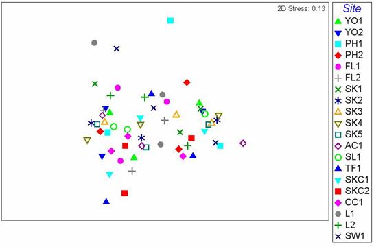
Table 2.8 Fish Family
Composition (%) During the Wet Season
|
Family |
YO1 |
YO2 |
PH1 |
PH2 |
FL1 |
FL2 |
SK1 |
SK2 |
SK3 |
SK4 |
SK5 |
AC1 |
SL1 |
TF1 |
SKC1 |
SKC2 |
CC1 |
L1 |
L2 |
SW1 |
|
Ambassidae |
26.7 |
25.5 |
15.2 |
29.7 |
11.9 |
14.2 |
18.0 |
22.8 |
29.7 |
26.4 |
26.2 |
34.9 |
29.5 |
15.8 |
23.0 |
22.7 |
25.4 |
18.7 |
22.9 |
56.3 |
|
Antennariidae |
0.0 |
0.0 |
0.0 |
0.0 |
0.0 |
0.0 |
0.0 |
0.0 |
0.0 |
0.0 |
0.0 |
0.0 |
0.1 |
0.1 |
0.0 |
0.0 |
0.0 |
0.0 |
0.6 |
0.0 |
|
Apogonidae |
0.1 |
0.3 |
0.2 |
0.4 |
0.6 |
0.4 |
1.8 |
0.4 |
0.7 |
0.2 |
0.8 |
0.5 |
0.5 |
3.5 |
2.3 |
2.1 |
4.6 |
2.0 |
1.7 |
0.9 |
|
Blenniidae |
0.9 |
2.0 |
0.3 |
1.0 |
1.5 |
0.5 |
1.1 |
2.1 |
2.6 |
0.5 |
1.3 |
1.0 |
0.2 |
1.5 |
0.7 |
1.2 |
4.2 |
6.7 |
5.9 |
2.8 |
|
Bothidae |
0.0 |
0.0 |
0.0 |
0.0 |
0.0 |
0.0 |
0.1 |
0.1 |
0.0 |
0.2 |
0.0 |
0.0 |
0.0 |
0.0 |
0.0 |
0.0 |
0.0 |
0.1 |
0.1 |
0.0 |
|
Bregmacerotidae |
0.8 |
1.2 |
0.4 |
1.4 |
0.6 |
3.7 |
7.5 |
3.1 |
1.9 |
2.6 |
2.7 |
3.5 |
0.8 |
0.4 |
2.2 |
2.2 |
0.3 |
4.4 |
3.3 |
1.8 |
|
Callionymidae |
0.0 |
0.1 |
0.5 |
0.2 |
1.1 |
0.1 |
0.3 |
0.2 |
0.4 |
0.1 |
0.2 |
0.5 |
0.5 |
0.3 |
0.2 |
0.2 |
0.5 |
0.4 |
0.3 |
0.3 |
|
Carangidae |
0.0 |
0.1 |
0.1 |
0.2 |
0.1 |
0.1 |
0.9 |
0.3 |
0.1 |
0.1 |
0.1 |
0.3 |
0.0 |
0.1 |
0.1 |
0.6 |
0.1 |
0.0 |
0.0 |
0.2 |
|
Clupeidae |
0.8 |
0.3 |
0.0 |
3.9 |
0.1 |
0.2 |
0.7 |
0.1 |
0.1 |
0.1 |
0.7 |
0.1 |
0.2 |
0.0 |
0.0 |
0.2 |
0.2 |
0.1 |
0.3 |
0.3 |
|
Cynoglossidae |
6.5 |
4.1 |
0.9 |
6.7 |
5.5 |
9.1 |
5.3 |
2.2 |
4.4 |
3.6 |
4.7 |
2.9 |
3.0 |
7.5 |
8.3 |
4.0 |
5.4 |
4.3 |
7.5 |
3.6 |
|
Drepaneidae |
0.1 |
0.1 |
0.0 |
0.1 |
0.2 |
0.0 |
1.0 |
0.4 |
0.2 |
0.1 |
0.0 |
0.1 |
0.1 |
0.1 |
0.0 |
0.2 |
0.1 |
0.4 |
0.6 |
0.2 |
|
Engraulidae |
22.8 |
19.9 |
58.2 |
22.4 |
30.4 |
14.4 |
18.3 |
15.6 |
21.4 |
22.6 |
12.5 |
10.5 |
24.2 |
26.6 |
19.3 |
11.8 |
8.9 |
16.2 |
18.8 |
6.1 |
|
Gerreidae |
0.0 |
0.0 |
0.0 |
0.0 |
0.1 |
0.0 |
0.1 |
0.1 |
0.1 |
0.0 |
0.2 |
0.0 |
0.0 |
0.0 |
0.0 |
0.1 |
0.0 |
0.0 |
0.0 |
0.0 |
|
Gobiidae |
14.3 |
13.9 |
8.2 |
13.9 |
15.0 |
22.9 |
6.4 |
16.1 |
9.0 |
17.8 |
14.1 |
11.3 |
15.7 |
16.8 |
16.8 |
27.7 |
21.1 |
17.4 |
17.4 |
9.4 |
|
Haemulidae |
0.2 |
0.1 |
0.0 |
0.0 |
0.0 |
0.1 |
0.5 |
0.3 |
0.0 |
0.0 |
0.3 |
0.1 |
0.0 |
0.0 |
0.0 |
0.0 |
0.0 |
0.3 |
0.0 |
0.1 |
|
Labridae |
0.0 |
0.0 |
0.0 |
0.0 |
0.0 |
0.0 |
0.2 |
0.0 |
0.0 |
0.0 |
0.0 |
0.0 |
0.0 |
0.0 |
0.0 |
0.0 |
0.0 |
0.1 |
0.0 |
0.0 |
|
Leiognathidae |
1.5 |
2.4 |
4.0 |
2.5 |
6.9 |
4.3 |
12.7 |
5.4 |
5.5 |
3.7 |
6.0 |
7.0 |
3.5 |
3.3 |
4.6 |
3.5 |
5.0 |
1.9 |
3.3 |
3.4 |
|
Lobotidae |
0.0 |
0.0 |
0.0 |
0.0 |
0.0 |
0.0 |
0.1 |
0.0 |
0.0 |
0.0 |
0.0 |
0.0 |
0.0 |
0.0 |
0.0 |
0.0 |
0.0 |
0.0 |
0.0 |
0.0 |
|
Monacanthidae |
0.0 |
0.0 |
0.0 |
0.1 |
0.4 |
0.0 |
0.1 |
0.1 |
0.0 |
0.1 |
0.2 |
0.2 |
0.1 |
0.1 |
0.5 |
0.2 |
0.1 |
3.5 |
0.1 |
0.4 |
|
Mugilidae |
0.2 |
0.1 |
0.1 |
0.1 |
0.2 |
0.0 |
0.2 |
0.1 |
0.2 |
0.5 |
0.9 |
0.6 |
0.1 |
0.7 |
0.7 |
0.3 |
0.6 |
1.6 |
0.6 |
0.0 |
|
Muraenidae |
0.0 |
0.0 |
0.0 |
0.0 |
0.0 |
0.1 |
0.2 |
0.0 |
0.0 |
0.0 |
0.1 |
0.0 |
0.0 |
0.0 |
0.0 |
0.0 |
0.0 |
0.0 |
0.1 |
0.0 |
|
Ophichthidae Eel |
0.0 |
0.1 |
0.0 |
0.1 |
0.1 |
0.0 |
0.1 |
0.0 |
0.0 |
0.2 |
0.0 |
0.2 |
0.0 |
0.0 |
0.3 |
0.0 |
0.2 |
0.0 |
0.0 |
0.0 |
|
Platycephalidae |
0.0 |
0.1 |
0.2 |
0.1 |
3.3 |
1.1 |
2.3 |
1.5 |
0.5 |
0.4 |
0.6 |
0.8 |
0.4 |
0.3 |
0.0 |
0.0 |
0.3 |
0.7 |
0.4 |
0.1 |
|
Pomacentridae |
0.0 |
0.0 |
0.0 |
0.0 |
0.0 |
0.0 |
0.1 |
0.0 |
0.0 |
0.0 |
0.0 |
0.0 |
0.0 |
0.0 |
0.0 |
0.0 |
0.0 |
0.1 |
0.1 |
0.0 |
|
Scaridae |
0.0 |
0.0 |
0.0 |
0.0 |
0.1 |
0.0 |
0.3 |
0.0 |
0.0 |
0.0 |
0.0 |
0.0 |
0.0 |
0.1 |
0.0 |
0.0 |
0.1 |
0.2 |
0.0 |
0.0 |
|
Scatophagidae |
0.0 |
0.0 |
0.0 |
0.0 |
0.0 |
0.0 |
0.0 |
0.0 |
0.0 |
0.0 |
0.0 |
0.0 |
0.0 |
0.0 |
0.0 |
0.0 |
0.1 |
0.1 |
0.1 |
0.0 |
|
Sciaenidae |
23.7 |
27.9 |
11.1 |
16.0 |
20.4 |
25.8 |
18.8 |
27.5 |
21.0 |
20.0 |
26.7 |
23.3 |
19.8 |
20.8 |
16.8 |
21.5 |
22.3 |
17.2 |
14.6 |
12.3 |
|
Scorpaenidae |
0.0 |
0.0 |
0.0 |
0.0 |
0.0 |
0.0 |
0.0 |
0.0 |
0.0 |
0.0 |
0.0 |
0.0 |
0.0 |
0.0 |
2.4 |
0.0 |
0.0 |
0.0 |
0.0 |
0.0 |
|
Serranidae |
0.0 |
0.0 |
0.0 |
0.0 |
0.1 |
0.0 |
0.5 |
0.1 |
0.0 |
0.0 |
0.1 |
0.0 |
0.0 |
0.0 |
0.0 |
0.0 |
0.0 |
0.1 |
0.0 |
0.1 |
|
Sillaginidae |
0.6 |
0.5 |
0.4 |
0.5 |
0.6 |
0.8 |
1.0 |
0.8 |
0.9 |
0.3 |
0.5 |
0.7 |
0.6 |
0.7 |
0.1 |
0.4 |
0.4 |
0.3 |
0.2 |
0.7 |
|
Soleidae |
0.0 |
0.0 |
0.0 |
0.0 |
0.0 |
0.0 |
0.1 |
0.0 |
0.0 |
0.0 |
0.0 |
0.0 |
0.0 |
0.0 |
0.0 |
0.0 |
0.0 |
0.0 |
0.0 |
0.0 |
|
Sparidae |
0.0 |
0.1 |
0.0 |
0.1 |
0.0 |
0.0 |
0.1 |
0.0 |
0.0 |
0.0 |
0.0 |
0.0 |
0.0 |
0.0 |
0.0 |
0.0 |
0.1 |
0.0 |
0.0 |
0.0 |
|
Synanceiidae |
0.2 |
0.3 |
0.1 |
0.2 |
0.3 |
0.2 |
0.1 |
0.1 |
0.1 |
0.1 |
0.1 |
0.1 |
0.3 |
0.0 |
0.3 |
0.4 |
0.0 |
0.4 |
0.2 |
0.3 |
|
Syngnathidae |
0.0 |
0.0 |
0.0 |
0.0 |
0.0 |
0.0 |
0.0 |
0.0 |
0.0 |
0.0 |
0.0 |
0.0 |
0.0 |
0.0 |
0.1 |
0.0 |
0.0 |
0.0 |
0.1 |
0.1 |
|
Synodontidae |
0.1 |
0.3 |
0.0 |
0.5 |
0.5 |
1.4 |
1.0 |
0.4 |
0.7 |
0.2 |
0.5 |
0.7 |
0.2 |
1.0 |
1.1 |
0.4 |
0.1 |
2.4 |
0.7 |
0.3 |
|
Terapontidae |
0.0 |
0.1 |
0.0 |
0.0 |
0.0 |
0.1 |
0.2 |
0.0 |
0.0 |
0.0 |
0.0 |
0.0 |
0.0 |
0.0 |
0.0 |
0.0 |
0.1 |
0.0 |
0.0 |
0.1 |
|
Tetraodontidae |
0.0 |
0.1 |
0.0 |
0.0 |
0.0 |
0.0 |
0.0 |
0.0 |
0.1 |
0.0 |
0.1 |
0.0 |
0.0 |
0.1 |
0.0 |
0.0 |
0.0 |
0.0 |
0.2 |
0.0 |
|
Trichiuridae |
0.0 |
0.1 |
0.0 |
0.1 |
0.1 |
0.0 |
0.0 |
0.2 |
0.2 |
0.1 |
0.2 |
0.1 |
0.0 |
0.0 |
0.1 |
0.0 |
0.0 |
0.3 |
0.1 |
0.1 |
|
Unidentified |
0.0 |
0.1 |
0.1 |
0.0 |
0.1 |
0.6 |
0.2 |
0.1 |
0.1 |
0.1 |
0.2 |
0.1 |
0.0 |
0.1 |
0.1 |
0.0 |
0.0 |
0.2 |
0.0 |
0.0 |
|
Total in each
station |
100 |
100 |
100 |
100 |
100 |
100 |
100 |
100 |
100 |
100 |
100 |
100 |
100 |
100 |
100 |
100 |
100 |
100 |
100 |
100 |
2.1.5
Day/Night-Surface/Bottom Surveys (July and
August 2005)
Stations SK1, SK2, SK3, SK4, and SK5 were each sampled by horizontal
tows using a closing ring net to investigate if there were any differences between
day and night samples collected from surface or bottom layers (Table 2.9).
Table
2.9 Mean Fish and Fish egg
densities (± SD) of Day/Night-Surface/Bottom Surveys
|
Station |
Type of survey |
Fish Density (larvae m-3) |
Fish Egg Density (egg m-3) |
|
SK1 |
Day-Surface |
16.253 (± 2.519) |
2.189 (± 3.821) |
|
Day-Bottom |
10.500 (± 1.863) |
0.668 (± 0.915) |
|
|
Night-Surface |
37.865 (± 5.947) |
1.529 (± 2.520) |
|
|
Night-Bottom |
31.332 (± 3.395) |
0.102 (± 0.131) |
|
|
SK2 |
Day-Surface |
14.573 (± 3.296) |
7.403 (± 13.503) |
|
Day-Bottom |
3.997 (± 0.832) |
3.710 (± 5.398) |
|
|
Night-Surface |
10.305 (± 1.818) |
1.731 (± 2.277) |
|
|
Night-Bottom |
2.883 (± 0.193) |
1.175 (± 2.099) |
|
|
SK3 |
Day-Surface |
0.145 (± 0.097) |
0.697 (± 0.780) |
|
Day-Bottom |
0.379 (± 0.404) |
0.262 (± 0.299) |
|
|
Night-Surface |
0.780 (± 0.492) |
1.106 (± 1.544) |
|
|
Night-Bottom |
0.609 (± 0.373) |
0.297 (± 0.341) |
|
|
SK4 |
Day-Surface |
1.098 (± 1.195) |
2.227 (± 2.700) |
|
Day-Bottom |
0.466 (± 0.466) |
1.386 (± 1.633) |
|
|
Night-Surface |
0.928 (± 0.615) |
43.116 (± 67.506) |
|
|
Night-Bottom |
1.346 (± 1.205) |
73.079 (± 92.486) |
|
|
SK5 |
Day-Surface |
1.010 (± 1.772) |
0.708 (± 0.991) |
|
Day-Bottom |
0.532 (± 0.574) |
0.407 (± 0.575) |
|
|
Night-Surface |
0.632 (± 0.692) |
2.737 (± 2.926) |
|
|
Night-Bottom |
0.951 (± 0.598) |
8.595 (± 10.313) |
The data collected and analysed highlighted no significant differences
between fish densities at any of the five stations around
It has to be noted that during the day/night – surface/bottom data
review a high density of Gobiidae and Bregmacerotidae were found in SK1 and
SK2.
Fish egg density, fish density, fish diversity and fish family
composition were identified and analysed from samples in the dry season (November
to March). Methodology
for data analysis was the same as the wet season as stated in Section 2.1.
2.2.1
Fish Egg Density
Due to the quantitative nature of the fish egg density survey, the results
presented combine the data of both the ichthyoplankton and fish post-larvae
samples as fish eggs were also collected in the post-larvae sampling nets.
The fish egg densities ranged from 0.161 ±0.565 egg m-3 in
CC1 to 4.382 ± 23.424 egg m-3 in FL2 (Table 2.10 and Figure 2.7).
Result of Two-Way ANOVA test showed that mean rank of fish egg density was
significantly different between months and between sampling stations (p =
0.05). Subsequent SNK test showed that mean rank of fish egg density in March was
significantly higher than that in February which was in turn significantly
higher than those in December, January and November. Stations at
Table
2.10 Mean Fish Egg Density (± SD)
(egg m-3) in the Dry Season
|
Station |
Dry Season |
|
YO1 |
0.761 (± 1.976) |
|
YO2 |
0.404 (± 1.242) |
|
PH1 |
0.846 (± 2.916) |
|
PH2 |
1.436 (± 5.340) |
|
FL1 |
0.357 (± 0.742) |
|
FL2 |
4.382 (± 23.424) |
|
SK1 |
1.161 (± 4.000) |
|
SK2 |
0.456 (± 1.335) |
|
SK3 |
0.617 (± 1.811) |
|
SK4 |
1.078 (± 3.208) |
|
SK5 |
0.496 (± 1.141) |
|
AC1 |
0.936 (± 3.011) |
|
SL1 |
0.674 (± 1.551) |
|
TF1 |
0.855 (± 2.218) |
|
SKC1 |
0.873 (± 3.635) |
|
SKC2 |
2.058 (± 8.419) |
|
CC1 |
0.161 (± 0.565) |
|
L1 |
0.282 (± 1.108) |
|
L2 |
0.299 (± 1.073) |
|
SW1 |
0.221 (± 0.649) |
Figure 2.7 Mean
Fish Egg Density – Dry Season. Two-Way ANOVA test indicated significant
differences in mean rank of fish egg density among 20 sampling stations (df =
19, f value = 3.674) and among months (df = 4, f value = 120.097).

Table 2.11 Main
results of SNK tests showing significant differences in mean rank of fish egg
density between sampling stations and between months in the Dry Season.
|
|
Significant difference between (1)
sampling stations and (2) between months (greatest to smallest, left to right) |
|
1. |
SK4, YO1, SK5, FL1, YO2, SL1, SK3, PH1, SK2, SK1, TF1, FL2, AC1 |
|
|
YO1
L1, PH2 |
|
|
SK5 CC1,
SKC1 |
|
|
FL1
SW1, L1, SKC2 |
|
2. |
MAR
> FEB > DEC = JAN = NOV |
2.2.2
Fish Density
Mean fish density was calculated using post larvae data collected in
both the ichthyoplankton survey nets and the post-larvae survey nets (I-net and
P-net respectively). The data were not
combined due to the quantitative and qualitative nature of the post larvae
assessment and are therefore presented separately (Table 2.12).
Table
2.12 Mean Fish Density (± SD)
(larvae m-3) in Ichthyoplankton and Fish Post-Larvae Surveys – Dry
Season
|
Station |
Ichthyoplankton |
Fish Post-Larvae |
|
YO1 |
0.296 (± 0.449) |
0.061 (± 0.134) |
|
YO2 |
0.108 (± 0.126) |
0.059 (± 0.096) |
|
PH1 |
0.134 (± 0.199) |
0.063 (± 0.083) |
|
PH2 |
0.276 (± 0.349) |
0.057 (± 0.067) |
|
FL1 |
0.258 (± 0.281) |
0.107 (± 0.141) |
|
FL2 |
0.292 (± 0.432) |
0.125 (± 0.195) |
|
SK1 |
0.280 (± 0.384) |
0.048 (± 0.078) |
|
SK2 |
0.148 (± 0.173) |
0.034 (± 0.069) |
|
SK3 |
0.190 (± 0.305) |
0.023 (± 0.028) |
|
SK4 |
0.124 (± 0.225) |
0.019 (± 0.023) |
|
SK5 |
0.217 (± 0.128) |
0.063 (± 0.120) |
|
AC1 |
0.159 (± 0.133) |
0.037 (± 0.050) |
|
SL1 |
0.219 (± 0.294) |
0.038 (± 0.046) |
|
TF1 |
0.212 (± 0.381) |
0.043 (± 0.043) |
|
SKC1 |
0.133 (± 0.182) |
0.029 (± 0.036) |
|
SKC2 |
0.149 (± 0.216) |
0.032 (± 0.026) |
|
CC1 |
0.199 (± 0.360) |
0.051 (± 0.088) |
|
L1 |
0.163 (± 0.245) |
0.047 (± 0.052) |
|
L2 |
0.243 (± 0.301) |
0.051 (± 0.095) |
|
SW1 |
0.164 (± 0.192) |
0.046 (± 0.060) |
Ichthyoplankton Survey
From a review of the post larvae data
collected with the ichthyoplankton survey it emerged that higher fish densities
were recorded in YO1, FL2, SK1 and PH2 with approximately 0.2 larvae m-3,
while the lowest fish density was 0.108 ± 0.126 larvae m-3 in YO2 (Table 2.12 and Figure 2.8). Result of Two-Way ANOVA test indicated that there was
significant difference in mean rank of fish density between months and between
sampling stations (p = 0.05). The mean rank of fish density in January was
significantly higher than those in December, November, February and March. For
the spatial difference, mean rank of fish density at SK5 was significantly
higher than that in SK4 (Table 2.13, p = 0.05).

Figure 2.8 Mean
Fish Density – Ichthyoplankton Survey. Two-Way ANOVA test indicated significant
differences in mean rank of fish density among 20 sampling stations (df = 19, f
value = 1.897) and among months (df = 4, f value = 23.148).
Table
2.13 Main
results of SNK tests showing significant differences in mean rank of fish
density between sampling stations and between months in the Dry Season.
|
|
Significant difference between (1)
sampling stations and (2) between months (greatest to smallest, left to right) |
|
1. |
SK5, PH2, FL1, SK1, AC1, FL2, YO1, SL1, L2, SK2, SK3, SW1, TF1, PH1,
L1, CC1, SKC2, SKC1, YO2 |
|
|
PH2
SK4 |
|
2. |
JAN
> DEC = NOV = FEB > MAR |
Fish
Post-Larvae Survey
From a review of the post larvae data
collected with the post-larvae net it emerged that the highest fish density was
recorded in FL2 with 0.125 ± 0.195 larvae m-3 (Table 2.12 and Figure 2.9)
. Result of Two-Way ANOVA test indicated that there was significant difference
in mean rank of fish density between months and between sampling stations (p =
0.05). The mean rank of fish density in January was significantly higher than
that in February which was in turn significantly higher than those in November,
December and March. For the spatial difference, mean rank of fish density at
FL1 was significantly higher than those at all other sampling stations (Table
2.14, p = 0.05).
Figure 2.9 Mean
Fish Density – Post-Larvae Survey. Two-Way ANOVA test indicated significant
differences in mean rank of fish density among 20 sampling stations (df = 19, f
value =3.384) and among months (df = 4, f value =88.047).

Table 2.14 Main
results of SNK tests showing significant differences in mean rank of fish
density between sampling stations and between months in the Dry Season.
|
|
Significant difference between (1)
sampling stations and (2) between months (greatest to smallest, left to right) |
|
1. |
FL1 |
|
|
PH1, PH2, FL2, TF1, YO2, SK5, SK1,
CC1, L2, SL1, L1, AC1, YO1, SKC2, SKC1, SW1, SK3, SK2, SK4 |
|
2. |
JAN
> FEB > NOV = DEC > MAR |
Seasonal Variation (November – March)
Fish post-larvae densities varied, showing a decrease in December but
then increased again in January (Table
2.15).
The results presented in Table
2.15 show that the highest fish densities (from both the ichthyoplankton
and post larvae nets) were obtained in January.
Lower densities were recorded in the remaining months, with the lowest
densities recorded in the March samples.
A similar trend was observed in the post larvae net samples.
Table
2.15 Mean Fish (larvae m-3)
and Fish egg (egg m-3) Densities in Ichthyoplankton and Fish
Post-Larvae Surveys in Each Sampling Period
|
Date |
Ichthyoplankton Survey |
Fish Post-Larvae Survey |
||
|
|
Fish Density (larvae m-3) |
Fish Egg Density (egg m-3) |
Fish Density (larvae m-3) |
Fish Egg Density (egg m-3) |
|
November
2005 |
0.149 |
0.125 |
0.037 |
0.002 |
|
December
2005 |
0.167 |
0.080 |
0.026 |
0.010 |
|
January
2006 |
0.453 |
0.157 |
0.147 |
0.023 |
|
February
2006 |
0.142 |
0.287 |
0.045 |
0.008 |
|
March
2006 |
0.080 |
8.441 |
0.007 |
0.044 |
2.2.3
Fish Post-Larvae Diversity
Since only the fish post-larvae collected with the post-larvae net were classified
to the family level, diversity of fish post-larvae which is represented by
number of family found and the Shannon-Wiener diversity index was calculated
only with this data set. The number of
family ranges from 8.40 ± 2.07 in CC1 to 13.00 ± 1.73 in FL1, whereas the
Shannon-Wiener diversity index ranged from 1.18 ± 0.36 in TF1 to 1.71 ± 0.19 in
FL2 (Table 2.16). Both number of family (Figure 2.10) and Shannon-Wiener index (Figure 2.11) showed no significant differences among the 20
sampling stations (One-Way ANOVA, p > 0.05).
Table 2.16 Mean
number of fish family (± SD) (larvae m-3) and Shannon-Wiener Index
recorded from Fish post-larvae Surveys – Dry Season
|
Stations |
No. of fish family recorded |
Shannon-Wiener Index |
|
|
|
|
YO1 |
10.80 (± 0.84) |
1.55 (± 0.24) |
|
|
|
|
YO2 |
9.80 (± 3.35) |
1.48 (± 0.36) |
|
|
|
|
PH1 |
11.40 (± 3.68) |
1.51 (± 0.55) |
|
|
|
|
PH2 |
11.80 (± 3.19) |
1.43 (± 0.24) |
|
|
|
|
FL1 |
13.00 (± 1.73) |
1.36 (± 0.37) |
|
|
|
|
FL2 |
12.00 (± 4.69) |
1.71 (± 0.19) |
|
|
|
|
SK1 |
11.00 (± 1.58) |
1.43 (± 0.50) |
|
|
|
|
SK2 |
10.00 (± 2.83) |
1.33 (± 0.52) |
|
|
|
|
SK3 |
11.20 (± 4.09) |
1.52 (± 0.63) |
|
|
|
|
SK4 |
9.80 (± 2.05) |
1.45 (± 0.65) |
|
|
|
|
SK5 |
12.80 (± 3.27) |
1.50 (± 0.56) |
|
|
|
|
AC1 |
12.20 (± 2.59) |
1.51 (± 0.58) |
|
|
|
|
SL1 |
10.20 (± 2.28) |
1.37 (± 0.57) |
|
|
|
|
TF1 |
9.60 (± 3.36) |
1.18 (± 0.36) |
|
|
|
|
SKC1 |
9.80 (± 1.48) |
1.48 (± 0.48) |
|
|
|
|
SKC2 |
10.60 (± 3.05) |
1.55 (± 0.38) |
|
|
|
|
CC1 |
8.40 (± 2.07) |
1.40 (± 0.44) |
|
|
|
|
L1 |
11.20 (± 2.68) |
1.43 (± 0.54) |
|
|
|
|
L2 |
11.00 (± 3.39) |
1.26 (± 0.48) |
|
|
|
|
SW1 |
10.20 (± 2.86) |
1.21 (± 0.55) |
|
|
|
Figure 2.10 Mean Number of Fish Family Recorded – Fish Post- Larvae
Survey. No significant difference in mean
number of fish family recorded was found among 20 sampling stations (n = 400,
df = 19) by One-Way ANOVA (F value = 0.80, p > 0.05)

Figure
2.11 Mean Shannon-Wiener Index – Fish Post- Larvae Survey. No significant difference in mean rank of
Shannon-Wiener Index was found among 20 sampling stations (n = 400, df = 19) by
One-Way ANOVA (F value =
0.35, p > 0.05)

2.2.4
Fish Family Composition
The families recorded for the dry season samples differed markedly from that
in wet season, with Callionymidae (Dragonets), Gobiidae, Scorpaenidae
(rockfishes) and Syngnathidae (pipefishes) replacing Ambassidae (glass
perches), Engraulidae (anchovies) and Sciaenidae (croakers) as the most common
families (Table 2.17). From the MDS plot, there was no apparent
spatial difference in fish family composition among the 20 sampling stations (Figure 2.12). It is supported by the subsequent ANOSIM
test, which could not reveal any significant difference in fish family
composition amongst the sampling stations (p > 0.05).
Figure
2.12 MDS
plot showing difference in fish family composition among sites in the Dry
Season. ANOSIM analysis indicated that
no significant difference in fish family composition was found among sites
(Global R =-0.10, p > 0.05)
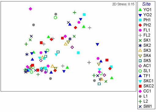
Table 2.17 Fish Family Composition (%) - Dry Season
|
Family |
YO1 |
YO2 |
PH1 |
PH2 |
FL1 |
FL2 |
SK1 |
SK2 |
SK3 |
SK4 |
SK5 |
AC1 |
SL1 |
TF1 |
SKC1 |
SKC2 |
CC1 |
L1 |
L2 |
SW1 |
|
Ambassidae |
0.0 |
0.2 |
0.4 |
0.1 |
0.1 |
0.0 |
0.0 |
0.0 |
0.2 |
0.0 |
0.2 |
0.2 |
0.1 |
0.0 |
0.0 |
0.0 |
0.0 |
0.2 |
0.0 |
0.0 |
|
Apogonidae |
0.8 |
0.3 |
0.5 |
0.4 |
0.3 |
0.1 |
0.3 |
0.3 |
0.2 |
0.7 |
0.1 |
0.5 |
0.7 |
0.4 |
0.3 |
0.2 |
0.2 |
0.3 |
0.1 |
0.1 |
|
Blenniidae |
0.9 |
0.9 |
0.9 |
1.1 |
0.8 |
1.0 |
5.9 |
4.9 |
2.7 |
4.2 |
2.9 |
2.5 |
1.1 |
0.6 |
1.1 |
3.6 |
0.5 |
3.8 |
6.5 |
3.2 |
|
Bothidae |
0.2 |
0.0 |
0.0 |
0.0 |
0.0 |
0.2 |
0.3 |
0.3 |
0.3 |
0.5 |
1.0 |
0.3 |
0.0 |
0.1 |
0.0 |
0.2 |
0.0 |
0.0 |
0.0 |
0.1 |
|
Bregmacerotidae |
0.5 |
0.2 |
0.5 |
0.3 |
0.0 |
0.3 |
0.6 |
4.5 |
2.7 |
2.8 |
10.5 |
2.6 |
2.8 |
0.3 |
3.1 |
1.8 |
3.0 |
3.8 |
9.0 |
7.5 |
|
Callionymidae |
3.9 |
7.0 |
5.1 |
7.9 |
4.8 |
9.8 |
6.0 |
6.5 |
4.3 |
3.0 |
9.2 |
11.7 |
6.9 |
6.0 |
8.0 |
9.0 |
14.6 |
14.6 |
12.7 |
5.8 |
|
Carangidae |
0.1 |
0.0 |
0.0 |
1.1 |
0.2 |
0.7 |
0.9 |
0.5 |
2.2 |
2.6 |
1.6 |
2.1 |
0.5 |
0.3 |
0.7 |
0.2 |
0.2 |
0.3 |
0.6 |
0.1 |
|
Centrolophidae |
0.0 |
0.0 |
0.2 |
0.0 |
0.0 |
0.0 |
0.0 |
0.0 |
0.0 |
0.0 |
0.0 |
0.0 |
0.1 |
0.0 |
0.0 |
0.2 |
0.2 |
0.2 |
0.0 |
0.0 |
|
Clupeidae |
0.1 |
0.3 |
0.7 |
0.5 |
0.4 |
0.5 |
0.3 |
0.7 |
0.3 |
0.5 |
0.0 |
0.8 |
0.5 |
0.3 |
0.7 |
0.8 |
0.3 |
0.7 |
0.8 |
0.3 |
|
Cynoglossidae |
1.0 |
0.0 |
0.5 |
0.2 |
0.1 |
0.1 |
1.5 |
0.0 |
0.2 |
0.0 |
0.5 |
0.2 |
0.2 |
0.0 |
0.3 |
0.0 |
0.0 |
0.2 |
1.1 |
0.4 |
|
Drepaneidae |
0.1 |
0.0 |
0.0 |
0.0 |
0.0 |
0.0 |
0.0 |
0.0 |
0.0 |
0.0 |
0.1 |
0.0 |
0.0 |
0.0 |
0.0 |
0.2 |
0.2 |
0.0 |
0.2 |
0.0 |
|
Elopidae |
0.0 |
0.2 |
0.0 |
0.0 |
0.1 |
0.1 |
0.0 |
0.0 |
0.0 |
0.0 |
0.0 |
0.0 |
0.0 |
0.1 |
0.0 |
0.0 |
0.0 |
0.0 |
0.0 |
0.0 |
|
Engraulidae |
7.6 |
7.8 |
26.7 |
10.5 |
11.2 |
4.0 |
6.9 |
7.2 |
3.8 |
4.9 |
6.5 |
5.9 |
4.0 |
6.6 |
1.4 |
2.6 |
2.5 |
2.0 |
11.9 |
6.3 |
|
Gerreidae |
0.0 |
0.0 |
0.0 |
0.0 |
0.1 |
0.0 |
0.0 |
0.0 |
0.0 |
0.0 |
0.1 |
0.2 |
0.0 |
0.0 |
0.1 |
0.0 |
0.0 |
0.0 |
0.0 |
0.0 |
|
Gobiidae |
14.2 |
13.9 |
16.3 |
18.7 |
8.7 |
23.7 |
2.5 |
4.5 |
4.8 |
4.0 |
3.4 |
5.8 |
5.2 |
2.4 |
3.1 |
4.2 |
3.7 |
1.7 |
2.0 |
2.6 |
|
Haemulidae |
0.0 |
0.0 |
0.0 |
0.0 |
0.0 |
0.1 |
0.0 |
0.0 |
0.2 |
0.0 |
0.0 |
0.0 |
0.0 |
0.0 |
0.0 |
0.0 |
0.0 |
0.0 |
0.0 |
0.0 |
|
Labridae |
0.0 |
0.0 |
0.0 |
0.0 |
0.0 |
0.0 |
0.0 |
0.0 |
0.0 |
0.0 |
0.0 |
0.2 |
0.0 |
0.0 |
0.0 |
0.0 |
0.0 |
0.0 |
0.1 |
0.0 |
|
Leiognathidae |
0.1 |
0.0 |
3.8 |
0.2 |
0.4 |
0.1 |
0.1 |
0.2 |
0.0 |
0.0 |
0.0 |
0.2 |
0.0 |
0.0 |
0.0 |
0.2 |
0.0 |
0.3 |
0.0 |
0.0 |
|
Monacanthidae |
0.0 |
0.0 |
0.2 |
0.0 |
0.1 |
0.0 |
0.0 |
0.0 |
0.0 |
0.0 |
0.0 |
0.0 |
0.0 |
0.0 |
0.0 |
0.0 |
0.0 |
0.0 |
0.0 |
0.0 |
|
Mugilidae |
0.1 |
0.3 |
1.8 |
0.0 |
4.1 |
2.8 |
0.2 |
1.0 |
0.7 |
0.7 |
1.6 |
0.2 |
0.0 |
0.0 |
0.1 |
3.4 |
0.8 |
0.5 |
0.8 |
0.4 |
|
Ophichthidae Eel |
0.0 |
0.2 |
0.0 |
0.0 |
0.0 |
0.0 |
0.1 |
0.0 |
0.2 |
0.2 |
0.7 |
0.2 |
0.0 |
0.0 |
0.0 |
0.0 |
0.0 |
0.5 |
0.0 |
0.0 |
|
Paralichthyidae |
0.0 |
0.0 |
0.5 |
0.0 |
0.0 |
0.0 |
0.0 |
0.2 |
0.2 |
0.2 |
0.0 |
0.0 |
0.0 |
0.0 |
0.0 |
0.0 |
0.0 |
0.0 |
0.0 |
0.0 |
|
Percichthyidae |
2.2 |
4.4 |
0.2 |
0.8 |
1.6 |
1.9 |
2.6 |
0.9 |
1.2 |
0.5 |
1.0 |
1.2 |
0.9 |
1.5 |
2.4 |
3.6 |
3.2 |
3.0 |
1.6 |
1.1 |
|
Platycephalidae |
0.5 |
1.0 |
1.5 |
0.9 |
0.7 |
0.6 |
0.6 |
1.0 |
1.8 |
1.2 |
1.1 |
0.7 |
2.0 |
1.0 |
0.7 |
2.0 |
2.4 |
2.8 |
0.8 |
3.3 |
|
Pomacentridae |
0.0 |
0.0 |
0.0 |
0.0 |
0.0 |
0.1 |
0.0 |
0.0 |
0.0 |
0.0 |
0.0 |
0.0 |
0.0 |
0.0 |
0.0 |
0.0 |
0.0 |
0.0 |
0.0 |
0.0 |
|
Scaridae |
0.0 |
0.3 |
0.0 |
0.0 |
0.0 |
0.1 |
0.0 |
0.2 |
0.0 |
0.5 |
0.0 |
0.0 |
0.0 |
0.5 |
0.0 |
0.2 |
0.0 |
0.0 |
0.0 |
0.0 |
|
Scatophagidae |
0.0 |
0.0 |
0.0 |
0.0 |
0.0 |
0.0 |
0.0 |
0.0 |
0.0 |
0.0 |
0.0 |
0.2 |
0.0 |
0.0 |
0.0 |
0.0 |
0.0 |
0.0 |
0.0 |
0.0 |
|
Sciaenidae |
3.6 |
3.4 |
6.5 |
0.8 |
2.3 |
3.2 |
5.2 |
3.8 |
1.8 |
1.2 |
2.4 |
3.0 |
0.6 |
0.3 |
0.4 |
0.2 |
1.2 |
2.8 |
4.0 |
1.0 |
|
Scorpaenidae |
28.4 |
30.8 |
19.4 |
37.4 |
55.8 |
20.0 |
58.9 |
58.4 |
69.0 |
68.5 |
51.1 |
55.7 |
68.5 |
72.8 |
70.9 |
57.2 |
50.6 |
56.6 |
42.7 |
60.0 |
|
Sillaginidae |
0.3 |
0.3 |
0.9 |
0.6 |
0.4 |
0.1 |
0.2 |
0.2 |
0.2 |
0.2 |
0.0 |
0.3 |
0.2 |
0.0 |
0.1 |
0.6 |
1.0 |
0.5 |
0.7 |
0.4 |
|
Soleidae |
1.2 |
0.2 |
1.3 |
1.9 |
0.5 |
1.3 |
1.9 |
0.9 |
0.7 |
2.3 |
1.9 |
2.1 |
1.2 |
1.9 |
0.9 |
1.4 |
1.7 |
1.2 |
0.5 |
0.8 |
|
Sparidae |
0.0 |
0.9 |
0.9 |
0.0 |
0.0 |
0.0 |
0.0 |
0.0 |
0.0 |
0.0 |
0.0 |
0.0 |
0.0 |
0.0 |
0.0 |
0.0 |
0.0 |
0.3 |
0.0 |
0.0 |
|
Sphyraenidae |
1.4 |
2.2 |
0.5 |
1.7 |
0.4 |
1.4 |
2.1 |
2.3 |
1.0 |
0.2 |
2.4 |
1.0 |
2.0 |
2.3 |
2.0 |
3.6 |
6.9 |
2.3 |
3.2 |
5.0 |
|
Synanceiidae |
0.0 |
0.2 |
0.5 |
0.0 |
0.1 |
0.1 |
0.0 |
0.3 |
0.0 |
0.0 |
0.1 |
0.5 |
0.1 |
0.0 |
0.0 |
0.0 |
0.0 |
0.2 |
0.0 |
0.0 |
|
Syngnathidae |
32.6 |
24.5 |
8.9 |
13.9 |
6.1 |
27.0 |
1.8 |
0.5 |
0.3 |
0.7 |
0.2 |
1.2 |
1.8 |
2.0 |
3.1 |
3.6 |
6.4 |
0.3 |
0.0 |
0.0 |
|
Synodontidae |
0.1 |
0.0 |
0.0 |
0.2 |
0.2 |
0.0 |
0.1 |
0.0 |
0.0 |
0.0 |
0.0 |
0.2 |
0.1 |
0.0 |
0.0 |
0.0 |
0.0 |
0.2 |
0.0 |
0.3 |
|
Terapontidae |
0.1 |
0.0 |
0.0 |
0.1 |
0.1 |
0.0 |
0.1 |
0.0 |
0.0 |
0.2 |
0.1 |
0.0 |
0.0 |
0.1 |
0.0 |
0.0 |
0.0 |
0.0 |
0.2 |
0.6 |
|
Tetraodontidae |
0.2 |
0.2 |
0.2 |
0.1 |
0.3 |
0.1 |
0.0 |
0.3 |
0.5 |
0.0 |
0.5 |
0.3 |
0.4 |
0.4 |
0.1 |
1.0 |
0.0 |
0.3 |
0.1 |
0.3 |
|
Trichiuridae |
0.0 |
0.2 |
0.2 |
0.1 |
0.0 |
0.0 |
0.0 |
0.0 |
0.0 |
0.0 |
0.2 |
0.0 |
0.0 |
0.0 |
0.0 |
0.0 |
0.3 |
0.0 |
0.0 |
0.0 |
|
Triglidae |
0.0 |
0.0 |
0.2 |
0.0 |
0.0 |
0.0 |
0.0 |
0.2 |
0.0 |
0.0 |
0.0 |
0.0 |
0.0 |
0.0 |
0.0 |
0.0 |
0.0 |
0.0 |
0.0 |
0.1 |
|
Unidentified |
0.0 |
0.2 |
0.5 |
0.4 |
0.2 |
0.6 |
0.8 |
0.0 |
0.8 |
0.2 |
0.4 |
0.3 |
0.0 |
0.1 |
0.1 |
0.2 |
0.0 |
0.3 |
0.2 |
0.1 |
|
Total in each
station |
100 |
100 |
100 |
100 |
100 |
100 |
100 |
100 |
100 |
100 |
100 |
100 |
100 |
100 |
100 |
100 |
100 |
100 |
100 |
100 |
3
FINDINGS
From an analysis of the data recorded in this Ichthyoplankton and Fish
Post-Larvae Survey it emerges that fish and fish egg densities recorded for all
of the sampling stations are generally low and that there is significant
difference in the densities among sites. However, the degrees of difference in
densities are small and this ultimately highlights that there is no observable
difference between fish or fish egg densities of the waters of the identified
spawning/nursery grounds for commercial fisheries of the southern waters of
Hong Kong and those of
Seasonal variation was detected as overall fish densities decreased
significantly after October and implied that the peak spawning period for most
fishes in southern waters of
In total, 40 different families have been recorded to date (Table 3.1). The majority of the fishes included gobies and
blennies (the latter consisting mainly of Osmobranchus elegans). However, the families occurring in highest
abundance in summer included: Ambassidae, Engraulidae, Gobiidae and
Sciaenidae. In winter, families
occurring in highest densities included Callionymidae, Gobiidae, Scorpaenidae
and Syngnathidae (pipefishes).
Table
3.1 Checklist of Fish Families
Recorded During the Surveys
|
N. |
Family |
Common Name |
|
1 |
Ambassidae |
Glass perch |
|
2 |
Apogonidae |
Cardinalfishes |
|
3 |
Blenniidae |
Blennies |
|
4 |
Bregmacerotidae |
Codlets |
|
5 |
Bothidae |
Lefteye flounder |
|
6 |
Callionymidae |
Dragonets |
|
7 |
Carangidae |
Jacks and trevallies |
|
8 |
Centrolophidae |
Warehou or rudderfish |
|
9 |
Clupeidae |
Herrings |
|
10 |
Cynoglossidae |
Tonguefishes |
|
11 |
Drepaneidae |
Spotted sicklefishes |
|
12 |
Elopidae |
Tenpounder |
|
13 |
Engraulidae |
Anchovies |
|
14 |
Gerreidae |
Silver biddies |
|
15 |
Gobiidae |
Gobies |
|
16 |
Haemulidae |
Grunts |
|
17 |
Latidae |
Barramundi cod |
|
18 |
Leiognathidae |
Ponyfishes |
|
19 |
Monacanthidae |
Leatherjackets or filefishes |
|
20 |
Mugilidae |
Mullets |
|
21 |
Muraenidae |
Moray eels |
|
22 |
Ophichtidae |
Eels |
|
23 |
Percichthyidae |
Basses |
|
24 |
Platycephalidae |
Flatheads |
|
25 |
Pomacentridae |
Damselfishes |
|
26 |
Scaridae |
Parrotfishes |
|
27 |
Scatophagidae |
Drums |
|
28 |
Sciaenidae |
Croakers |
|
29 |
Scorpaenidae |
Rockfishes |
|
30 |
Sillaginidae |
Sillagos or sand borers |
|
31 |
Soleidae |
Soles |
|
32 |
Sparidae |
Snapper |
|
33 |
Sphyraenidae |
Barracudas |
|
34 |
Synanceiidae |
Stonefishes |
|
35 |
Syngnathidae |
Pipefishes and seahorses |
|
36 |
Synodontidae |
Lizardfishes or |
|
37 |
Terapontidae |
Grunters or tigerperches |
|
38 |
Tetraodontidae |
Pufferfishes |
|
39 |
Trichiuridae |
Cutlassfishes |
|
40 |
Triglidae |
Searobins |
Species richness tended to be higher, with maximum 23 to 30 families
were found in one station during summer (July-October), but decreased to about maximum
14 to 17 families in one station during winter (November-March).