1
Introduction
This annex covers the details of the
Quantitative Risk Assessment (QRA) for the Gas Receiving Station (GRS) at the
Black Point Power Station (BPPS) which will receive gas through the subsea pipeline from the South Soko
LNG Terminal . Detailed information of the study is
presented here whilst the results and conclusions are given in the main report,
Section 13.
2
Design Details
The pipeline from the South Soko Terminal to the BPPS
will terminate at a GRS. For the detailed layout of the GRS, see Figure 3.10 of Section 3 of the main report.
The GRS will be located on a plot of 100m
by 50m and comprise the following facilities:
·
2
emergency shutdown (ESD) valves
·
1 pig
receiver, with associated service piping;
·
Station
inlet header;
·
2
inlet filter-separators (plus 1 standby);
·
2
metering runs (plus 1 standby);
·
4
water bath gas heaters (plus 1 standby);
·
2
pressure control runs (plus 1 standby);
·
Station
export header and check valves.
Piping and equipment will be skid-mounted
and placed on prepared concrete footings. Larger piping and equipment
assemblies will be delivered to site as discreet subassemblies and assembled
on-site. Sensitive instrumentation will be housed in air-conditioned instrument
enclosures that are commonly prefabricated portable buildings.
Gas will be received via the offshore
pipeline and the first major piece of equipment in the station will be an
Emergency Shutdown (ESD) valve, which can be closed by means of the station ESD
system in the event of an emergency, isolating the station from the source of
gas.
Downstream of the ESD valve will be the
station inlet header that will distribute the gas to inlet filter units.
Parallel to the inlet filters oriented in-line with the incoming pipeline will
be a pig receiver, enabling the running of cleaning and inspection pigs in the
pipeline.
3
Population Data
Both land and marine populations are considered in the analysis. Two
cases are considered; years 2011 and 2021.
3.1
Land Population Estimation
The
following information sources were referred to for population estimation:
·
Site Survey Data [1]
·
Population Survey Report [2]
·
Census Data [3]
·
Land Records from Lands Department
·
Road Traffic Data [4]
·
Data on Key Individual Developments
·
Marine Traffic Data [5-7]
As
a conservative assumption, a radius of 2km from the boundary of the proposed
GRS has been considered for population estimation (Figure 3.1). The land population is assumed to be the same for
years 2011 and 2021.
Figure 3.1 Population
in the Vicinity of Black Point
3.1.1
Industrial Population
According to data provided by Planning
Department, Lung
Kwu Sheung Tan and the
government land allocated for temporary use (part of TPU 432) are the only
areas assumed to hold population within 2km radius of the GRS [9]. The
Table 3.1 Industrial
Facility Population
|
Location |
Approx. Distance from GRS |
2011 Population |
2021 Population |
|
Black Point Site Surrounding |
1km |
100 |
100 |
3.1.2
Road Traffic Population
Access
to Black Point Power Station is via
The population.. estimation for
No. of persons =
(AADT x Vehicle Occupancy / 24 / Speed)
=
4,380 x 3 / 24 / 50 = 11 persons/km
The traffic along this section of road has
increased at an average rate of 4.3% in recent years. Assuming this trend
continues, the traffic will increase by 30% by the year 2011, and by 100% by
the year 2021. The future population for both 2011 and 2021 is therefore
conservatively estimated as 11 x 2 = 22 persons/km.
3.1.3
Occupancy and Indoor/Outdoor Fractions
The land population is categorised further
into 4 time periods: night time, weekday, peak hours and weekend day. These are
defined in Table 3.2.
Table 3.2 Population
Time Periods
|
Time Period |
Description |
|
Night
time Weekday Peak
hours Weekend
day |
7:00pm to 7:00am 9:00am to 5:00pm Monday through Friday,
and 9:00am to 1:00pm Saturday 7:00am to 9:00am and 5:00pm to 7:00pm,
Monday to Friday 7:00am to 9:00am and 1:00pm to 3:00pm,
Saturdays 3:00pm to 7:00pm Saturdays, and 7:00am
to 7:00pm Sundays |
The occupancy assumed [2] during these
time periods is given in Table 3.3.
Different occupancy figures are assumed for industrial, residential and road
types of population. The proportion of the population outdoors is also assumed
to vary according to type of population and time period (Table 3.3).
The hazards that can potentially affect
offsite population are flash fires and thermal radiation from pool fires.
Buildings are assumed to offer protection to its occupants for these events.
The protection factor used is 90%, or equivalently the exposure factor is 10%.
Scenarios are therefore assumed to affect 100% of the outdoor population and
10% of the indoor population.
Road vehicles are also assumed to offer
some protection, although less than a building. An exposure factor of 50% is
used for vehicles.
Table 3.3 Land
Population Occupancy and Indoor/Outdoor Fractions
|
Population |
Occupancy |
% Outdoors |
||||||
|
Type |
Night |
Peak |
Weekday |
Weekend day |
Night |
Peak |
Weekday |
Weekend day |
|
Industrial Residential Road |
10 % 100 % 10 % |
10 % 50 % 100 % |
100 % 20 % 50 % |
10 % 80 % 20 % |
5 % 0 % 0 % |
10 % 30 % 0 % |
10 % 10 % 0 % |
10 % 20 % 0 % |
3.2
Marine Population
Estimation
Black Point is situated near
3.2.1
Vessel Population
The vessel population used in this study
are as given in Table 3.4. The
figures are based on BMT’s Marine Impact Assessment
report [6] except those for fast ferries. The maximum population of fast
ferries is assumed to be 450, based on the maximum capacity of the largest
ferry operating in
Table 3.4 Vessel
Population
|
Type of Vessel |
Average Population per Vessel |
% of Trips |
|
Ocean-Going
Vessel Rivertrade Coastal vessel Fast
Ferries Tug
and Tow Others |
21 5 450
(largest ferries with max population) 350
(typical ferry with max population) 280
(typical ferry at 80% capacity) 175
(typical ferry at 50% capacity) 105
(typical ferry at 30% capacity) 35
(typical ferry at 10% capacity) 5 5 |
3.75 3.75 22.5 52.5 12.5 5.00 |
3.2.2
Marine Vessel Protection Factors
The population on marine vessels is
assumed to have some protection from the vessel structure, in a similar way
that buildings offer protection to their occupants. The degree of protection
offered depends on factors such as:
·
Size
of vessel
·
Construction
material and likelihood of secondary fires
·
Speed
of vessel and hence its exposure time to the flammable cloud
·
The
proportion of passengers likely to be on deck or in the interior of the vessel
·
The
ability of gas to penetrate into the interior of the vessel and achieve a
flammable mixture.
Small vessels such as fishing boats will
provide little protection but larger vessels such as ocean-going vessels will
provide greater protection. Fast ferries are air conditioned and have a limited
rate of air exchange with the outside. Based on these considerations, the
fatality probabilities assumed for each type of vessel are as given in Table 3.5.
Table 3.5 Population
at Risk
|
Marine Vessel Type |
Population |
Fatality Probability |
Population at Risk |
|
Ocean-Going
Vessel Rivertrade Coastal Vessel Fast
Ferries Tug
and Tow Others |
21 5 450 350 280 175 105 35 5 5 |
0.1 0.3 0.3 0.3 0.3 0.3 0.3 0.3 0.9 0.9 |
2 2 135 105 84 53 32 11 5 5 |
3.2.3
Methodology
In this study, the marine traffic
population in the vicinity of Black Point has been considered as both point
receptors and average density values. The population of all vessels are treated
as an area average density except for fast ferries which are treated as point
receptors.
The marine area around Black Point was
divided into 12.67km2 grid cells, each grid being approximately
3.6km x 3.6km. The transit time for a vessel to traverse a grid is calculated based
on the travel distance divided by the vessel’s average speed. The average speed
[5] and transit time for different vessel types are presented in Table 3.6.
Table 3.6 Average Speed and Transit Time of
Different Vessel Type [5]
|
Type of Vessel |
Assumed Speed (m/s) |
Transit Time (min) |
|
Ocean-going vessel |
6.0 |
9.9 |
|
Rivertrade
Coastal vessel |
6.0 |
9.9 |
|
Fast Ferries |
15.0 |
4.0 |
|
Tug and Tow |
2.5 |
23.7 |
|
Others |
6.0 |
9.9 |
|
|
|
|
The number of vessels traversing each grid
daily was provided by the marine consultant [5]. These are given in Table 3.7, where the grid cell reference
numbers are defined according to Figure
3.2. The number of marine vessels present within each grid cell at any
instant in time is then calculated from:
Number
of vessels = No. of vessels per day x grid length / 86400 / Speed
(1)
This was calculated for each type of
vessel, for each grid and for years 2011 and 2021. The values obtained
represent the number of vessels present within a grid cell at any instant in
time. Values of less than one are interpreted as the probability of a vessel
being present.
Figure 3.2 Grid
Cell Numbering Scheme
Table 3.7 Number
of Marine Vessels Per Day
|
Grid No. |
Average Number of Vessels Per Day |
|||||||||
|
2011 |
2021 |
|||||||||
|
OG |
RT |
TT |
FF |
OTH |
OG |
RT |
TT |
FF |
OTH |
|
|
1 2 3 4 |
19 0 19 0 |
788 0 557 368 |
368 21 263 168 |
44 0 77 11 |
567 84 294 294 |
23 0 23 0 |
863 0 610 403 |
403 23 288 184 |
52 0 91 13 |
621 92 322 322 |
OG = Ocean-going vessels
RT = Rivertrade
coastal vessels
TT = Tug & tow vessels
FF = Fast ferries
OTH = others
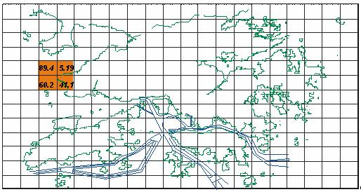
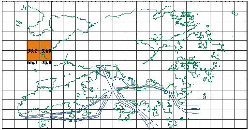
Average
Density Approach
The average
marine population for each grid is calculated by combining the number of vessels
in each grid (from Equation 1) with the population at risk for each
vessel (Table 3.5). The results are shown in Figures 3.3 and 3.4.
This grid population is assumed to apply to all time periods. Note however that
fast ferries are excluded since ferries are treated separately in the analysis
(see below).
When simulating
a possible release scenario, the impact area is calculated from dispersion
modelling. In general, only a fraction of the grid area is affected and hence
the number of fatalities within a grid is calculated from:
Number of fatalities = grid population x impact area / grid
area (2)
Figure 3.3 Marine Population at Risk by Grid, Year
2011
Figure
3.4 Marine Population at Risk by
Grid, Year 2021
Point
Receptor Approach
The
average density approach, described above, effectively dilutes the population
over the area of the grid. Given that ferries have a much higher population
than other classes of vessel, combined with a relatively low presence factor
due to their higher speed, the average density approach would not adequately
highlight the impact of fast ferries on the FN curves. Fast
ferries are therefore treated a little differently in the analysis.
In reality, if a fast ferry is affected by
an accident scenario, the whole ferry will likely be affected. The likelihood
that the ferry is affected, however, depends on the size of the hazard area and
the density of ferry vessels. To model this, the population is treated as a
concentrated point receptor i.e. the entire population of the ferry is assumed
to remain focused at the ferry location. The ferry density is calculated the
same way as described above (Equation 1),
giving the number of ferries per grid at any instant in time, or equivalently a
“presence factor”. A hazard scenario, however, will not affect a whole grid,
but some fraction determined by the area ratio of the hazard footprint area and
the grid area. The presence factor, corrected by this area ratio is then used
to modify the frequency of the hazard scenario:
Prob.
that ferry is affected = presence
factor x impact area / grid area (3)
The fast ferry population distribution
adopted was described in Table 1.5.
Information from the main ferry operators suggests that 25% of ferry trips take
place at night time, while 75% occur during daytime. Day and night ferries are
therefore assessed separately in the analysis. The distribution assumed is
given in Table 3.8.
Table 3.8 Fast
Ferry Population Distribution for Day and Night Time Periods
|
Population |
Population at Risk |
% of Day Trips |
% of Night Trips |
% of All Trips (= 0.75 x day + 0.25 x night) |
|
450 350 280 175 105 35 |
135 105 84 53 32 11 |
5 5 30 60 - - |
- - - 30 50 20 |
3.75 3.75 22.5 52.5 12.5 5.0 |
The ferry presence factor (Equation 1) and probability that a ferry
is affected by a release scenario (Equation
2) are calculated for each ferry occupancy category and each time period.
3.2.4
Stationary Marine Population
Stationary marine population in the vicinity
of the GRS was also considered. Contributions to these populations come from
the
Figure 3.5 Stationary
Marine Population at Risk (2011)

Figure 3.6 Stationary
Marine Population at Risk (2021)
4
Meteorological Data
Data on local meteorological conditions such as wind speed, wind
direction, atmospheric stability class, ambient temperature and humidity was
obtained from the Hong Kong Observatory.
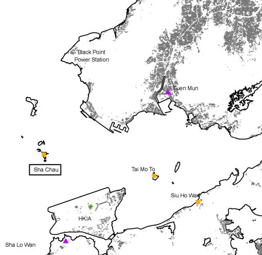
The location of weather stations in the vicinity of the GRS is shown in Figure 4.1. Data from the Sha Chau weather station was
adopted for the GRS study as it is closest to the site and also the most
relevant based on the topography. The meteorological data used in this study is
based on the data recorded by the stations over a five year period.
Figure 4.1 Weather
Stations in Vicinity of Black Point
The raw data from the Observatory is a series of readings taken every
hour for a period of one year. This data has been rationalized into different
combinations of wind direction, speed and atmospheric stability class, as per
the following:
·
Each
data record is rated with a stability class A through F. For simplicity, this
study has used three stability classes, B, D and F. Accordingly, the data
records have been assigned to these three classes;
·
Each
data record has an associated wind speed. For simplicity, this study has used
five wind speed classes. Accordingly, the data records have been assigned to
these five classes;
·
Each
data record has an associated wind direction. For simplicity, this study has
used 12 wind directions. Accordingly, the data records have been assigned to
these twelve classes;
·
The
data has been split into night and day times encompassing day time from 7am to
7pm and night time from 7pm to 7am.
The annual average temperature for Black Point is 23.9 °C. Temperature data was not available from
the Sha Chau station and so
temperature readings were taken from the
Table 4.1 Temperature
Statistics for Black Point
|
|
|
Min. |
Max. |
Average |
|
Ambient air (T°C)1 |
BP |
6.7 |
35.1 |
23.9 |
|
Surface (T°C)1 |
|
20.9 |
25.7 |
23 |
|
Seawater (T°C)2 |
BP |
16.2 |
27.8 |
23.9 |
|
Humidity (%)1 |
|
65 |
82 |
77 |
Source: 1.
2. HK EPD, “Summary water quality statistics of the
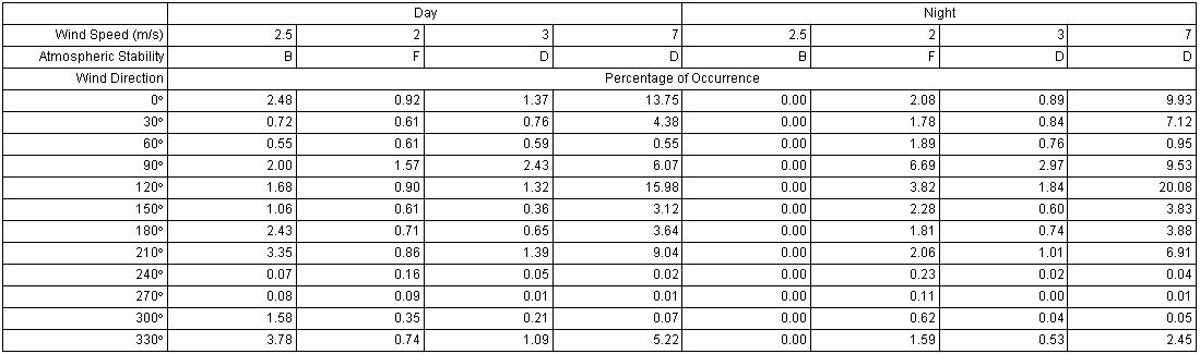
The percentage of occurrence for each combination of wind direction,
speed and atmospheric stability during day and night are presented in Table
4.2. In addition, the percentages frequencies are plotted in the form of
wind roses for Sha Chau in Figure
4.2.
Wind directions, such as 90°, refer to the direction of the prevailing
wind. For example, 90° refer to an easterly wind, 0° is northerly, 180° is southerly and 270° is westerly.
Table 4.2 Data
for Sha Chau Weather
Station
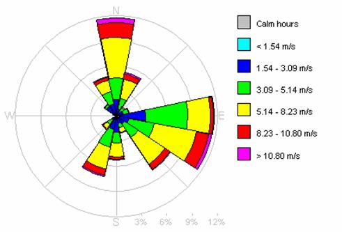
Figure
4.2 Wind Rose for Sha Chau Weather Station
(1999-2004)
Note on Atmospheric
Stability
The Pasquill-Gifford atmosphere stability
classes range from A through F.
A: Turbulent
B: Very
unstable
C: Unstable
D: Neutral
E: Stable
F: Very
stable
Wind speed and solar radiation interact to determine the level of
atmospheric stability, which in turn suppresses or enhances the vertical
element of turbulent motion. The latter is a function of the vertical
temperature profile in the atmosphere; the greater the rate of decrease in
temperature with height, the greater the level of turbulence.
Class A represents extremely unstable conditions, which typically occur
under conditions of strong daytime insolation.
Category D is neutral and neither enhances nor suppresses atmospheric
turbulence. Class F on the other hand represents moderately stable conditions,
which typically arise on clear nights with little wind.
5
Frequency Analysis
Failure Frequencies
Table 5.1 lists all the failure frequencies adopted for the
various release scenarios used in the GRS study. Codes are assigned for various
source terms; these are defined in Section
6, Table 6.1.
Table 5.1 Gas
Release Event Frequencies
|
No. of Items |
Length of Section (m) |
Hole Size (mm) |
Initiating Event Frequency |
Unit |
Reference |
|
|
G1 |
1 |
25.5 |
10 |
1.00E-07 |
per meter per year |
Hawksley [5] |
|
|
|
|
25 |
1.00E-07 |
|
|
|
|
|
|
50 |
7.00E-08 |
|
|
|
|
|
|
100 |
7.00E-08 |
|
|
|
|
|
|
FB |
3.00E-08 |
|
|
|
G2 |
4 |
4.5 |
10 |
3.00E-07 |
per year |
Hawksley |
|
|
|
|
25 |
3.00E-07 |
||
|
|
|
|
50 |
1.00E-07 |
||
|
|
|
|
100 |
1.00E-07 |
||
|
|
|
|
FB |
5.00E-08 |
||
|
G3 |
2 |
3.9 |
10 |
3.00E-07 |
per meter per year |
Hawksley |
|
|
|
|
25 |
3.00E-07 |
|
|
|
|
|
|
50 |
1.00E-07 |
|
|
|
|
|
|
100 |
1.00E-07 |
|
|
|
|
|
|
FB |
5.00E-08 |
|
Ignition Probabilities
Table 5.2 gives a summary of the ignition probabilities
assumed for the study. 10 and 25mm holes are considered “small leaks”, while 50
and 100mm holes are considered “large leaks”.
Table 5.2 Ignition
Probabilities Assumed
|
|
Immediate Ignition |
Delayed Ignition 1 |
Delayed Ignition 2 |
Delayed Ignition Probability |
Total Ignition Probability |
|
Gas small leak |
0.02 |
0.045 |
0.005 |
0.05 |
0.07 |
|
Gas large leak/rupture |
0.1 |
0.2 |
0.02 |
0.22 |
0.32 |
Outcome Frequencies
A Generic Event Trees is shown in Figure
5.1. Based on the initiating event frequencies listed in Table 5.1 and ignition probabilities in Table 5.2, specific event trees can be
generated for different release scenarios.
Figure 5.1 Generic
Event Tree
|
|
Detection and Shutdown Fails |
Immediate Ignition |
Delayed Ignition (1) |
Delayed Ignition (2) |
Event Outcome |
|
||||
|
Release |
Yes |
|
Yes |
|
|
|
|
|
Jet Fire/Fireball |
JTF_IF |
|
|
No |
|
No |
|
|
|
|
|
|
|
|
|
|
|
|
|
Yes |
|
|
|
Flash Fire over Plant Area |
FF1_IF |
|
|
|
|
|
|
No |
|
|
|
|
|
|
|
|
|
|
|
|
|
Yes |
|
Flash Fire Full Extent |
FF2_IF |
|
|
|
|
|
|
|
|
No |
|
|
|
|
|
|
|
|
|
|
|
|
|
Unignited Release |
NE |
|
|
|
|
|
|
|
|
|
|
|
|
|
|
|
|
Yes |
|
|
|
|
|
Jet Fire/Fireball |
JTF_IS |
|
|
|
|
No |
|
|
|
|
|
|
|
|
|
|
|
|
|
Yes |
|
|
|
Flash Fire over Plant Area |
FF1_IS |
|
|
|
|
|
|
No |
|
|
|
|
|
|
|
|
|
|
|
|
|
Yes |
|
Flash Fire Full Extent |
FF2_IS |
|
|
|
|
|
|
|
|
No |
|
|
|
|
|
|
|
|
|
|
|
|
|
Unignited Release |
NE |
|
|
|
|
|
|
|
|
|
|
|
|
A summary of outcome frequencies for all the events considered in the
GRS study is listed in Table 5.3.
Detail of the nomenclature is as follows:
IS = Isolation Success
IF = Isolation
Failure
FF1 = Flash
Fire over the Plant Area
FF2 = Flash
Fire, Full Extent
PLF = Pool
Fire
JTF = Jet Fire
FBL = Fire
Ball
FB = Full Bore
NE = No Effect
Table 5.3 Outcome
Frequencies Summary
|
Release Event |
Release Scenario |
|
|
|
|
|
|
|
10mm |
25mm |
50mm |
100mm |
IS_FB |
IF_FB |
|
G01_FF2 |
4.68E-11 |
4.68E-11 |
1.01E-10 |
1.01E-10 |
3.89E-10 |
4.32E-11 |
|
G01_FF1 |
4.41E-10 |
4.41E-10 |
1.26E-09 |
6.93E-09 |
4.86E-09 |
5.40E-10 |
|
G01_JTF |
2.00E-10 |
2.00E-10 |
7.00E-10 |
7.00E-09 |
|
3.00E-10 |
|
G01_FBL |
|
|
|
|
2.70E-09 |
|
|
G02_FF2 |
1.40E-10 |
1.40E-10 |
1.44E-10 |
1.44E-10 |
6.48E-10 |
7.20E-11 |
|
G02_FF1 |
1.32E-09 |
1.32E-09 |
1.80E-09 |
9.90E-09 |
8.10E-09 |
9.00E-10 |
|
G02_JTF |
6.00E-10 |
6.00E-10 |
1.00E-09 |
1.00E-08 |
|
5.00E-10 |
|
G02_FBL |
|
|
|
|
4.50E-09 |
|
|
G03_FF2 |
1.40E-10 |
1.40E-10 |
1.44E-10 |
1.44E-10 |
6.48E-10 |
7.20E-11 |
|
G03_FF1 |
1.32E-09 |
1.32E-09 |
1.80E-09 |
9.90E-09 |
8.10E-09 |
9.00E-10 |
|
G03_JTF |
6.00E-10 |
6.00E-10 |
1.00E-09 |
1.00E-08 |
|
5.00E-10 |
|
G03_FBL |
|
|
|
|
4.50E-09 |
|