contents
1 Introduction............................................................................................................ 1-1
2 Summary
And conclusions.................................................................................. 2-1
3 CLIMATIC
AND HYDROGRAPHIC FEATURES............................................................ 3-1
3.1 Climatic
Features........................................................................................................... 3-1
3.2 Hydrographic
Features................................................................................................... 3-1
3.2.1 Tide................................................................................................................................. 3-1
4 HYDROGRAPHIC
DATA BASIS.................................................................................... 4-1
4.1 Reference
System......................................................................................................... 4-1
4.2 Bathymetric
Information................................................................................................. 4-1
4.3 Water
Levels.................................................................................................................. 4-3
4.4 Current
and Salinity........................................................................................................ 4-3
4.5 Wind............................................................................................................................... 4-4
4.6 River
Discharge............................................................................................................. 4-5
5 Model
set-up............................................................................................................ 5-1
5.1 Model
Areas.................................................................................................................... 5-1
5.1.1 Regional
model.............................................................................................................. 5-1
5.1.2 Inner
model areas.......................................................................................................... 5-3
5.1.3 New
Lung Kwu Chau models........................................................................................ 5-3
5.2 Culverts.......................................................................................................................... 5-6
5.3 Simulation
Periods......................................................................................................... 5-7
5.4 Model
Forcing................................................................................................................. 5-8
5.4.1 Tide................................................................................................................................. 5-8
5.4.2 Initial
and open boundary conditions.............................................................................. 5-8
5.4.3 River
discharge............................................................................................................ 5-10
5.4.4 Wind............................................................................................................................. 5-11
5.4.5 Tilting............................................................................................................................ 5-11
6 Simulation
results................................................................................................ 6-1
6.1 Model
verification............................................................................................................ 6-1
6.2 Influence
of the jetty........................................................................................................ 6-7
6.2.1 Tracer
experiment........................................................................................................ 6-11
6.3 Sediment
spill modelling.............................................................................................. 6-13
6.3.1 Construction
phase scenario....................................................................................... 6-13
6.3.2 Spreading
simulation results........................................................................................ 6-15
7 Environmental
Impact Assessment................................................................. 7-1
7.1 Water
Quality................................................................................................................. 7-1
7.2 Background
Conditions.................................................................................................. 7-1
7.3 Release
and Dispersal of Sediments............................................................................ 7-2
7.4 Chinese
White Dolphin................................................................................................ 7-12
7.5 Impact
on Benthic Organisms and Artificial Reefs...................................................... 7-13
7.6 Other
Impacts on Water Quality.................................................................................. 7-14
8 Morphological
Impact Assessment................................................................ 8-1
8.1 Description
of Problem.................................................................................................. 8-1
8.2 Study
Methodology......................................................................................................... 8-3
8.2.1 Yearly
mean wind-wave climate off the eastern coast of Lung Kwu Chau................... 8-4
8.2.2 Detailed
analysis of wave conditions in the vicinity of the project site........................... 8-7
8.3 Results
and Conclusions............................................................................................... 8-9
9 references.............................................................................................................. 9-1
Drawings
Drawing 1: Typical
current field (m/s) calculated in 675 m during neap period, outgoing flow
during dry season
Drawing 2: Typical
current flow (m/s) calculated in 675 m grid during neap tide, incoming
flow during dry season
Drawing 3: Grain
size distribution curve
1
Introduction
DHI Water & Environment undertakes
the numerical modelling of hydrodynamic and sediment spreading for the proposed
new Lung Kwu Chau Jetty as subconsultant to Maunsell Environmental Management
Consultants Ltd., Hong Kong.
The methodology for the study approach
has previously been described in the Methodology report for hydrodynamic and
sediment spreading, cf. Ref. /1/.
The present report describes the set-up
and execution of the local hydrodynamic and sediment spreading models used for
the study of the Lung Kwu Chau Jetty impact. Subsequently, assessment of the
impacts from the new jetty on the water quality and coastal morphology is
presented.
The local model has been set up to enable
simulations of currents and salinity in the Pearl River estuary based on the
model suite applied in the Pillar Point Study.
The model has been extended to include a
subset grid containing a nested
75 m - 25 m - 8.3 m dynamically linked grid
for simulations of currents around the new jetty. As part of these simulations,
two culverts are included in the catwalk, which form part of the jetty.
3D simulations have been performed for
both dry and wet season hydrodynamics.
The dry season is simulated as a period
during 1993, where the model previously has been calibrated against WAHMO data
sets. The wet season is simulated as a period during 1996, where SSDS EIA data
has been used for model calibration. The simulations have been compared to
previous results obtained in the Pillar Point study, and good agreement is observed.
The results imply that the model can be
used for description of the hydrodynamic regime around Lung Kwu Chau.
Simulations with the jetty and culverts
demonstrate a limited effect of the jetty on the overall flow regime and water
exchange in the bay north of the jetty. Furthermore, there will be virtually no
effect of the culverts.
Simulations with sediment spreading
demonstrate the excursion of the spill plume and the sedimentation to be
expected around Lung Kwu Chau. The simulation of sediment spreading form the
basis for the subsequent impact assessment.
Mitigation measures have been proposed to
minimize the water quality impact and comprise a dredging rate of 500 m3/day
and implementation of a silt curtain around the closed grab dredger. A higher dredging rate is proposed to reduce
the duration of impact of the dredging works on marine ecological receivers, in
particular the Chinese White Dolphin which is the key sensitive receiver in the
Marine Park. The highest levels of concentration
in the sediment plume are shown to remain close to the source. During mitigated dredging, the sediment
plumes would be very narrow and even in the plume, the concentrations of
suspended matter would, in general, be only slightly elevated. Furthermore, the surplus suspended matter
during the dredging works would be well below natural maximum suspended solids
concentrations measured in the assessment area, and the impact on water quality
would occur on a very local scale and transient nature.
Chinese White Dolphin
Considering the limited magnitude and the
local nature of the impact from the dredging operations on turbidity as well as
the large area in which the dolphins are distributed, the dolphins will hardly
experience the turbidity regime during the construction to deviate
substantially for the natural conditions. However, it cannot be totally
excluded that transient and local displacements will occur due to changes in
fish distribution caused by fish avoidance of the sediment plumes from the
dredging.
The potential threats to the dolphins
include habitat loss caused by extensive coastal development and reclamation,
intense boat traffic causing disturbance and collisions, incidental
entanglement in fishing gear, overfishing of prey species and pollution with
e.g. organoclorides such as PCB's and DDT.
Compared to these general threats, the
limited impact of the jetty construction on the water quality around Lung Kwu
Chau must be regarded as negligible, even considering the general pressure on the
dolphin population.
Impact on benthic organisms and artificial reefs
An artificial reef has been established
in the Marine Park about 2 km south of Lung Kwu Chau. A biological community
will develop or have already developed on this artificial reef. As was the case
for the fauna in the area in general, only species adapted to a rather high
turbidity will colonise the artificial reef. Furthermore, the model
calculations show that the artificial reef will be virtually unaffected by
sediment from the dredging operations. Therefore, no impact of the jetty
construction on the marine life on the artificial reef is expected. The same
conclusion is judged to be valid for the occurrences of Gorgonian soft corals
that have been observed at some locations near Tree Island and Sha Chau.
Morphological assessment
The potential impact that construction of
a jetty and dredging of an approach channel to a level of –2.5 m CD
in front of the berth at Lung Kwu Chau, Hong Kong, may have on the morphology
of the pocket beach located to the north of the project site has been assessed.
The assessment has been based on the
analysis of the changes that construction of the jetty and the dredging of the
channel will introduce in the wave conditions existing in front of the beach.
The rationale behind this approach is that
·
Unchanged wave conditions will
preserve a stable beach as it exists today
·
Significant gradients in wave height
along the beach due to the sheltering of the incident waves by the jetty will
generate currents capable of transporting sediment, thus impacting on the beach
morphology by changing its equilibrium alignment
Wave conditions in front of the beach
were determined through a two-step approach. First, the yearly mean wind-wave
climate off the eastern coast of Lung Kwu Chau was established by applying MIKE
21 NSW together with yearly wind statistics at Lau Fau Shan. Secondly, the wave
conditions in front of the beach were computed using MIKE 21 PMS for five
selected wave cases (combination of significant wave height Hm0,
peak period Tp and mean direction of wave propagation MWD). The
simulations considered both the existing situation and following construction
of the jetty and dredging of the channel.
The results obtained showed a relatively
mild yearly mean wave climate, in agreement with the protected location of the
island and the moderate wind conditions in the area.
It was also found that construction of
the jetty and dredging of the access channel will not significantly change the
wave conditions in front of the beach for the predominant (easterly) direction.
For waves approaching from more southerly directions (150°N and 170°N), the
jetty will have a relatively larger impact. However, the beach is to a large
extent sheltered from these waves by the rocky headland existing on its
southern side. Furthermore, large waves from southerly directions have
associated a very low probability of occurrence.
Based on the analysis and the results
summarised above, it is concluded that construction of the jetty and dredging
of the access channel to –2.5 m CD as projected will not impact
negatively on the morphology of the beach to the north of the project site.
3.1
Climatic Features
Hong Kong is situated in an area
dominated by the monsoons. Traditionally, the climatic year in South East Asia
is perceived as consisting of the south-west and north-east monsoons separated
by so-called transitional periods. A wet season, lasting from April to
September, and a dry season, lasting from October to March dominate the
climatic year.
From the monthly offshore wind roses in Figure 3.1 it is observed how October and January are dominated
by a strong north-east monsoon, while July exhibits a faint south-west monsoon
component, only. On the average, the January north-east component amounts to
7.1 m/s while the July south-west component amounts to 4.6 m/s.
3.2
Hydrographic Features
3.2.1
Tide
Numerous islands break up the bathymetry
around Hong Kong. The relatively large tidal ranges MHHW at 2.2 m and MLLW at
0.8 m give rise to complicated tidal circulation patterns in the Hong Kong
waters and the Pearl Estuary, cf. Figure
3.2. The tide is composed by both diurnal and semidiurnal
tides.
Out in the open South China Sea, the tide
is of a less complicated character. The tidal wave is entering the deep
northern part of the South China Sea through the Luzon strait. Having
progressed into relatively shallow water, the tidal wave bifurcates towards
north and south. On the south coast of China, the tidal stream appears to set
west on the rising tide and east on the falling tide at a mean rate of one
knot, Ref. /5/. Between the islands, speed and direction depend completely on
local bathymetric conditions.
From the numerous tide gauges situated
along the South Chinese Coast, numerous sets of tidal constituents have been
established. Ten sets of constituents are listed in Table 3.1. The stations are listed from west to east. A certain
gradual change in the constituents is observed, typically both the phase lag
and the amplitude decrease towards east. Possible deviations may be ascribed to
variations in the database for the constituent analysis. A short period
affected by unusual wind conditions may bias the analysis.
Tidal constituents represent a curve fit
to the astronomical tide experienced at a given gauge. Depending on the
duration of the underlying measurement series, the constituents represent
average tidal conditions at the location in question.
Figure 3.1 January, April, July and October offshore
wind roses in the area south of Hong Kong, Ref. /3/.
Figure 3.2 Hong Kong waters and the Pearl Estuary.
Table 3.1 Tidal constituents M2, S2, Kl & Ol at
various stations along the South Chinese Coast (Ref. /3/). The stations outside
inner Hong Kong waters are marked on Figure 5.1.
|
Station
|
No
|
M2
phase
Deg
|
Amp
H(m)
|
S2
phase
Deg
|
Amp
H(m)
|
K1
phase
Deg
|
Amp
H(m)
|
O1
phase
Deg
|
Amp
H(m)
|
|
Xiachuan Dao
|
7063
|
315
|
0.6
|
000
|
0.2
|
320
|
0.4
|
275
|
0.3
|
|
Gaolan Dao
|
7066
|
309
|
0.5
|
348
|
0.2
|
319
|
0.4
|
270
|
0.3
|
|
Wenwei Zhou
|
7087
|
275
|
0.3
|
305
|
0.1
|
302
|
0.3
|
255
|
0.3
|
|
Tai Mo To
|
7096
|
292
|
0.49
|
323
|
0.19
|
315
|
0.4
|
264
|
0.31
|
|
Tsing Yi
|
7102
|
271
|
0.42
|
296
|
0.17
|
296
|
0.36
|
253
|
0.29
|
|
Yung Shue Wan
|
7106
|
264
|
0.36
|
301
|
0.14
|
294
|
0.36
|
247
|
0.27
|
|
Hong Kong Harbour
|
7110
|
269
|
0.39
|
297
|
0.15
|
299
|
0.35
|
250
|
0.28
|
|
Waglan Island
|
7122
|
268
|
0.33
|
298
|
0.13
|
299
|
0.35
|
250
|
0.28
|
|
Hong Hai Wan
|
7145
|
250
|
0.3
|
277
|
0.1
|
293
|
0.4
|
247
|
0.2
|
|
Jiazi Jiao
|
7149
|
315
|
0.2
|
000
|
0.1
|
292
|
0.4
|
247
|
0.2
|
As the present Lung Kwu Chau Jetty model
is based on the model applied in the Pillar Point Study, Ref. /3/, the
following listing of hydrographic data pertain to the model calibration
performed during the Pillar Point study. The 900 m, 675 m and
225 m models applied in the present study are identical to the models
applied in the Pillar Point study, for which reason the data listed have been
applied in the model calibration for these models.
4.1
Reference System
The vertical datum of all bathymetric
information is the Chart Datum, which is 0.146 m below Principal Datum Hong
Kong.
Time is local Hong Kong time.
The positions are defined according to
the Hong Kong projection characterised by the
following parameters:
Centre: 114.1785556
Semi
Major Axis: 6,378,888.0
Semi
Minor Axis: 6,378,888.0
Scale: 1.0
Flatness:
0.003367
False
Easting: 836,695.0
False
Northing: -1,649,325,988
4.2
Bathymetric Information
The model area bathymetries (land-water
boundaries and water depths) for the various model sets are established from
·
Digitised depth information provided
by CED (WAHMO data)
·
Satellite images from 1989 and 1992
·
Topographical maps, Series HM50CL,
1990 and 1992. Crown Lands and Survey Office, Hong Kong
·
Updated bathymetry information from
new 1994 Chinese survey
·
Admiralty Charts
· EPD data around Lung Kwu Chau, received in 2002
The density and coverage of the
bathymetric information obtained during this study are indicated in Figure 4.1. A close-up of the density of bathymetric information
around the Island of Lung Kwu Chau is provided in Figure 4.2.
Figure 4.1 The density and coverage of bathymetric
information obtained during the present study. The position of the established
75 m grid is indicated.

Figure 4.2 A close-up of the density of bathymetric
information off the east coast of Lung Kwu Chau Island.
4.3
Water Levels
The following information on water levels
has been obtained in the calibration phase.
Royal Observatory of Hong Kong:
Amplitudes and phases of major constituents (30) used for tidal prediction in
Hong Kong. Constituents have been used from 8 stations: Chi Ma Wan, Lok On Pai,
Tai O, Tai Po Kau, Ko Lau Wan, Quarry Bay, Tsim Bei Tsui and Waglan island.
Environmental Protection Department, Hong
Kong: Deep Bay Water Quality Regional Control Strategy Study (by AXIS, CES,
Delft Hydraulics, etc.) Draft Pearl
Estuary Model Report, August 1996.
4.4
Current and Salinity
For the dry season simulations, the 1993
field survey campaign (named WHAMO) was used for calibration of the model
set-up.
The campaigns in 1993 included
measurements of current (speed and direction) over the water column during
approximately 30-hour periods in both spring and neap tide in a number of
stations in the area.
In order to perform a valid comparison of
simulated and measured current, the measured current is depth-averaged. This is
done by calculating the arithmetic mean of the vector components of the
measured current in the different sampling depths.
An extensive field campaign was performed
in the Hong Kong waters during the wet season in August-September 1996. During
this campaign, current (speed and direction) and salinity over the water column
were measured.
The campaign in 1996 (named SSDS EIA)
included measurements during approximately 30-hour periods in both spring and
neap tide distributed over a total period of approximately 9 days. The stations
are distributed spatially covering the Pearl Estuary, the inner Hong Kong
waters and some offshore areas.
The comparison between simulated and
measured variables (current and salinity) during the wet season was carried out
at two different depths: at the surface and at mid-depth, though they have been
measured at different levels over the vertical.
All comparison have been reported in the
Pillar Point study, cf. Ref. /3/.
4.5
Wind
The wind measurements applied in the
calibration for the wet season have been derived from the following stations:
1.
Green Island (GI)
2.
Hong Kong Observatory Headquarter
(HKO)
3.
Star Ferry (SF)
4.
Central (CEN)
5.
Hong Kong International Airport (SE
only) (AMO)
6.
Lau Fau Shan (LFS)
7.
Chek Lap KoK (CLK)
8.
Tuen Mun (TUN)
9.
Cheung Chau (CCH)
10. Waglan Island (WGI)
Time-series of wind speed and direction
for the wet season calibration period, i.e. end August through beginning of
September 1996, are depicted in Figure
4.3.

Figure 4.3 Time-series of wind speed and direction
in 8 selected stations during calibration period August-September 1996.
4.6
River Discharge
For the period of January 1993,
information on the river discharge was obtained from four outlets in the upper
section of the Pearl Estuary. These flow rates were obtained under the SSDS
Stage II study, cf. Ref. /2/.
For the period of August-September 1996,
information was obtained from China on the river discharge from eight outlets
in the Pearl Estuary. It has been assumed that the flow rates correspond to the
fresh water discharge, i.e. excluding tidal flows.
5.1
Model Areas
5.1.1
Regional model
The large regional 900 m model was
established to ensure that the tidal wave enters correctly among the numerous
islands around Hong Kong, see Figure
5.1. The regional model is forced by applying the tidal
water level from tidal station Xiachuan Dao (St. 7063) on the shore of the
western open boundary and Jiazi Jiao (St. 7149) on the shore of the eastern
open boundary. The objective is to deduce tidal constituents in the offshore
corner points of the regional model in order to make a tidal wave enter
correctly into the inner part of the regional model. The three open boundaries
of the regional model are forced by assuming a linear variation of the water
level between the shore stations and the offshore corner point. On the southern
offshore open boundary, the level variations are described linearly between the
western corner point and a so-called 'mid point' (co-ordinate 140,0) and the
level variations are described linearly between the mid point and the eastern
corner point. The background for this approach is the propagation of the tide,
i.e. the phase of the tide is not assumed to be linearly distributed along this
southern open boundary.
Characteristics of the regional model are
shown below:
Dx : 900 m
Dy : 900 m
Dimensions
(0:Nx) : 0 - 438
Dimensions
(0:Ny) : 0 - 255
Dimensions : 394 x 230 km2
Origin
(lat., long.) : 20.41615 o, 112.97144 o
Orientation
relative to North : - 20 o
Dt : 240 s
Figure 5.1 Regional model grid with a grid spacing
of 900 m. The model is aligned with the coast-line of southern China. Tidal
stations along the coast are indicated.
Figure 5.2 675 m intermediate grid area for execution of 2D and 3D
model simulations with local 225 m and detailed 75 m grids outlined.
5.1.2
Inner model areas
A set of inner model areas has been
established, according to the description outlined in the Methodology Report,
Ref. /1/.
The model set-up is configured as a
three-level dynamically nested grid system (Figure
5.2) with a 675 m grid, a 225 m intermediate
grid and two 75 m local grids. In this way, the model covers the entire
Hong Kong area, including the Pearl Estuary, and still resolves the flows of
Victoria Harbour and the adjacent straits and channels to a certain detail.
Details of the grids are given in Table 5.1.
Table 5.1 Hong Kong model grids.
|
Spacing
(m)
|
Dimension
(grid points)
|
Geographical
position
(lat.; long.)
|
Orientation
(deg. N)
|
|
675
|
242x172
|
21.78;112.99
|
-0.35
|
|
225
|
241x139
|
22.15;113.77
|
0
|
|
75
|
142x76
|
22.32;114.01
|
0
|
|
75
|
37x61
|
22.27;114.22
|
0.1
|
5.1.3
New Lung Kwu Chau models
A local nested model around Lung Kwu Chau
is introduced to enhance the resolution at Lung Kwu Chau. A 75 m,
25 m and 8.3 m nested grid area has been introduced to describe the
details of the hydrodynamics around the proposed new jetty, cf. Table 5.2.
Table 5.2 Local nested model around Lung Kwu Chau.
|
Spacing (m)
|
Dimension (grid
points)
|
Origo in enclosing
grid
|
|
75
|
51x84
|
30,40
|
|
25
|
42x57
|
14,48
|
|
8.3
|
42x45
|
19,21
|
The additional grid refinement is
necessary to resolve the proposed jetty, so that hydrodynamic conditions around
the jetty can be simulated.
The 75 m model domain covers the
entire area around Lung Kwu Chau and Sha Chau, while the 25 m grid area
covers the eastern side of Lung Kwu Chau Island and the 8.3 m grid area
covers the local area around the jetty.
Figure 5.3 Detailed 75 m and 25 m grids
around Lung Kwu Chau for description of hydrodynamic conditions around the Lung
Kwu Chau Jetty. The 8.3 m grid inside the 25 m grid is not included
for presentation purposes.
For description of local hydrodynamic
conditions around the proposed jetty, the
75 m - 25 m - 8.3 m model has been applied
using transferred boundaries from the larger 225 m model.
Two inner and internally dynamically
linked model complexes have thus be applied:
225 m - 75 m for
hydrodynamics in the Pearl River Estuary
75 m - 25 m - 8.3 m for description
of hydrodynamic conditions around the jetty and spreading of sediments
The full suite of models ranging from
675 m to 8.3 m has not been run dynamically, since the inclusion of
an 8.3 m horizontal resolution will increase the computational time. This
is due to the added nodes, but more significantly because of the reduced time
step to be applied in the model. The vertical resolution is set to be 2 m.
Figure 5.4 Bathymetric land contour applied in the
8.3 m model for the present situation relative to site plan, drawing
P20276-1B, Ref. /11/.
Figure 5.5 Bathymetric land contour applied in the
8.3 m model for new jetty. Relative to site plan, drawing P20276-1B, Ref.
/11/.
The jetty and the catwalk are located in
the innermost model grid, which has a grid spacing of 8.3 m. In this grid, the
jetty is represented by 2 grid points, which are both defined as land points.
The catwalk is represented by 2 grid points, which are defined as 'structure'
points with a north-south aligned culvert structure each. The representation of
the jetty and catwalk in the model grid is illustrated in Figure 5.5.
5.2
Culverts
Two culverts are placed in the catwalk to
enable a flow through the structure and minimise the impact of the structure on
the flow pattern, cf. Figure
5.6.
To enable a model description of the two
culverts placed in the catwalk, the model has been extended with the ability of
describing structures on the following basis:
The headloss, DH, over one culvert is given by:
 (Inflow + pipe
+ outflow)
(Inflow + pipe
+ outflow)
In which
V : velocity
L : length of jetty value: 15 m
M : Manning number value: 85 m1/3/s
R : hydraulic radius value: 0.19 m
G : gravitational acceleration value: 9.82 m2/s
The flux, Q, through one culvert is calculated as:
which, inserted in the previous equation,
provides a relationship between Q an H:

This enables a description of the flow
through a culvert in a single cell grid point based on the water level
difference over the cell. The water level difference between the ends of the
culverts (across the catwalk) will occur as a result of the tidal wave propagation
in the area, and the subsequent water level set-up in front of the jetty.
Figure 5.6 Plan of catwalk with culverts.
5.3
Simulation Periods
The simulation period has been chosen
identical to the calibration periods previously used in the Pillar Point study.
These were chosen based on available data from the monitoring campaigns
conducted in the Hong Kong Waters, described in Section 4.
Calibration has previously been conducted
on the following data sets and periods:
|
Corresponding
data sets
|
Year
|
Season
|
Simulation
period
|
|
SSDS
EIA
|
1996
|
Wet
|
27/8
- 5/9
|
|
WAHMO
|
1993
|
Dry
|
1/1 -
17/1
|
5.4
Model Forcing
The main forcing of the hydrodynamic
model consists of the tide, which was generated in the regional model and the
freshwater inflow from the Pearl River. Moreover, wind is included.
5.4.1
Tide
The calibration of the 900 m
regional model surrounding Hong Kong has required a long procedure due to the
very limited data available at the boundaries. Furthermore, these boundaries
are rather long (approximately 150 km for the west and east boundaries and 400
km for the south boundary), and the tidal propagation over the model domain is
complex. For example, the behaviour of the tide along the west and east
boundaries is different. In the first case, where the propagation is parallel
to the coastline, the phase differences are very small along the boundary; for
the east boundary the phases undergo an important variation due to propagation
with a large component towards the coast.
This also implies that within the model
domain, a large inflection in the tidal propagation has to happen, and there is
no data on which to base a detailed description of this phenomenon, as required
for an accurate calibration of a mathematical model. Therefore, to calibrate
the 900 m regional model it has been necessary to decompose the study of
the tidal propagation over the area and to perform a number of sensitivity
analyses, from which enough information could be generated to infer the correct
behaviour of the boundaries.
For the 900 m regional model, only
the further offshore stations (Tai O, Chi Ma Wan and Waglan Island) have been
considered. The other stations are analysed in the intermediate 675 m
model and finer grid models.
5.4.2
Initial and open boundary conditions
The 675 m model is forced on the
open lateral boundaries by water level variations at west and south and by
transfer boundary conditions (fluxes and levels) at east. These boundary
conditions have been extracted from the regional model. Applied as a
"boundary-condition-generator" for the wet season 3D model, the regional
model has been run using the same time variant and spatially constant wind as
in the 675 m model. Because the regional model supplies depth-averaged
(i.e. vertically constant) velocities, the vertical velocity profile at the
eastern model boundary has been improved by adding a parabolic wind term from
the surface and down to a depth of 20 metres:
where z is the vertical co-ordinate in
metres measured positive upwards from the sea surface, and U0 was chosen to be
3% of the wind speed. This term proved to be important in order to maintain the
eastern model boundary as an outflow boundary, consistent with the wind-driven
seasonal surface current.
Prior to the simulations, a 3D initial
salinity distribution has been established based on the available measurements
as well as on trial model runs during model calibration for the wet season.
This salinity field should provide the vertical and horizontal distribution in
consistency with the salinity at the boundaries (see below) as well as with the
wind-driven flow (see above). Also, the initial salinity field should in the
Pearl Estuary contain a sufficient amount of fresh water originating from river
inflows prior to the start of the simulation period. At the position of each
station, a vertical salinity profile has been interpolated from the
measurements to match the computational grid. Vertical profiles were
constructed in areas remote from the measurements, e.g. near the model
boundaries and in the northern part of the Pearl Estuary. All vertical salinity
profiles have then entered an objective analysis procedure to define a salinity
value at each computational grid point. The objective analysis has been
performed in the horizontal planes only so as not to damage the vertical
stratification. The salinity field has then been smoothed horizontally. Due to
insufficient amount of measurements, it has been necessary to perform
adjustments of the initial salinity field (e.g. shape and position of fronts)
as part of the model calibration.
The stratification in the model area
during the wet season is maintained through the river run-offs together with
the salinity boundary conditions. The baroclinic forcing at the open lateral
model boundaries is obtained from prescribed salinity distributions. Since there
has been no measured salinity data available to impose on the model boundaries,
the boundary salinity distributions have been part of the model calibration.
During the wet season, the eastward flowing, wind-generated current carries
brackish surface water into the model area from river outlets west of Macau. It
is important to include the oceanic current as well as the brackish (~5-15 psu)
water supply into the model, since otherwise the modelled salinities in the
Hong Kong area will be too much affected by the oceanic water (~34 psu)
flushing the area during flood. The salinity boundary conditions must be
adjusted to take this into account. This adjustment is, however, complicated
due to the very limited temporal and spatial coverage of measured salinities.
The final salinity boundary conditions may be schematically described as
follows: The salinity is oceanic, 34 psu, at all boundaries below a depth of
approximately 8 m. At the surface, a salinity of 32 psu is applied to the
north-eastern model boundary, decreasing to 25 psu at the south-eastern model
corner, to 16 psu at the south-western model corner and to 12 psu near the
coast at the western boundary.
5.4.3
River discharge
In the dry season simulations, the model
included 4 outlets of the Pearl River freshwater outflow. The flows applied in
the four outlets are shown in Table
5.3.
Table 5.3 Dry season fresh water inflow into Pearl
Estuary, 1993.
|
Model source
|
Distributary
|
Distribution of
Total flow
|
Discharge 1993 (m3/s)
|
Position in
675 m grid
|
|
1
2
3
4
|
Humen
Jiaomen
Hougqizhi
Hengmen
|
49%
37%
10%
4%
|
900
740
200
80
|
(95,169)
(88,157)
(91,134)
(84,131)
|
In the wet season model calibration, the
Pearl River fresh water inflow is described by eight model sources located in
the Pearl Estuary (Table
5.4).
The values of Table 5.4 have been calculated as average discharge values over
the periods of calibration for the simulation. It appears that the distribution
of the outflow for the eight tributaries follows a fixed relation with respect
to the upstream flow. These fixed relations (calculated as average values for
the simulation periods) are included in Table
5.4.
Table 5.4 Wet
season water inflow into Pearl Estuary.
|
Model source
|
Distributary
|
Percentage
(%)
|
Discharge
96 (m3/s)
|
Position in
675 m grid
|
|
1
2
3
4
5
6
7
8
|
Humen
Jiaomen
Hougqizhi
Hengmen
Modaomen
Jidimen
Hutiaomen
Yamen
|
18.5
17.3
6.4
11.2
28.3
6.1
6.2
6.0
|
3798
3551
1314
2299
5809
1254
1272
1231
|
(95,169)
(88,157)
(91,134)
(84,131)
(53,85)
(43,51)
(56,64)
(16,74)
|
5.4.4
Wind
It has been attempted to include the wind
based on recordings from the calibration periods during the wet season. The
purpose being partly to drive the offshore current while simultaneously
including the wind effects on the calculated current pattern in the area.
The wind has been applied as time variant
but simultaneously constant in space due to the high correlation between the
measurement stations. Time-series of averaged wind speed and directions over
the 10 available stations (see Section 4.5) have been applied to the model during the wet
season.
During dry season simulations, a
temporally constant wind field has been applied.
5.4.5
Tilting
In the calibration, it has been attempted
to include the offshore deep current by introducing a tilting of the boundary
in the regional model. In this manner, a unidirectional flow is imposed in the
model attaining current speed corresponding to the water level increase. A
water level difference of 0.50 m has been introduced between the eastern and
western boundaries (±0.25 m at the boundaries) of the regional model. As an
effect of the tilting, the water levels in the model are slightly distorted and
present an offset with the predicted water levels in the order of 0.20 - 0.25
m. This offset has to be considered and included in the water level results.
The tilting is intended to replace the
effect obtained by introducing an artificial wind field to drive the offshore
current.
6.1
Model verification
The results of the simulations with the
local model set-up have been compared to the results achieved during the Pillar
Point study. Hereby, verification of the model performance has been obtained.
Two points in the 75 m grid have
been selected, east and west of the Lung Kwu Chau Island, and current speed and
direction have been compared for the 75 m nested model with results
obtained in the 225 m model used during the Pillar Point study. The location
of the points are indicated in Figure
6.1.
The results for the dry season
simulations of this study are presented as 3D results, whereas previous results
were obtained in a 2D simulation. The success criterion for acceptable
performance is hence that the 3D results for current speed and direction are
centred around the previously obtained 2D results.
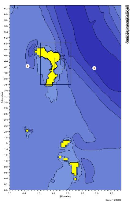
Figure 6.1 Position of two points (9,57) and (36,57)
for comparison of present study results with previous Pillar Point results.
Comparisons
of dry season simulations are shown in Figure
6.2 through Figure 6.7.
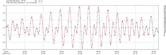
Figure 6.2 Comparison between previous calculated
water level results and presently calculated results in point (36,57) in the
75 m resolution. 17 days during dry season shown.
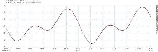
Figure 6.3 Comparison between previous calculated
water level results and presently calculated results in point (36,57) in the
75 m resolution. 2-day subset during dry season shown.
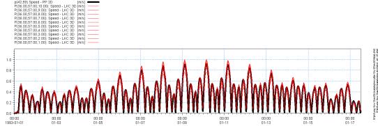
Figure 6.4 Comparison between previous calculated
current speed (depth averaged) and presently calculated speeds in point (36,57)
in the 75 m resolution. 17 days during dry season shown.
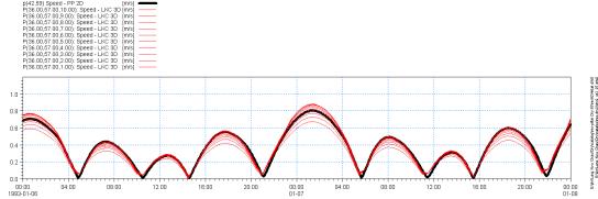
Figure 6.5 Comparison between previous calculated
current speed (depth averaged) and presently calculated speeds in point (36,57)
in the 75 m resolution. 2-day subset during dry season shown.
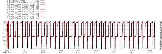
Figure 6.6 Comparison between previous calculated
current directions (depth averaged) and presently calculated directions in
point (36,57) in the 75 m resolution. 17 days during dry season shown.
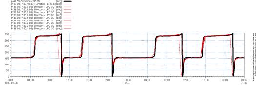
Figure 6.7 Comparison between previous calculated
current directions (depth averaged) and presently calculated directions in
point (36,57) in the 75 m resolution. 2-day subset during dry season
shown.
The results for the dry season show that
the calculated water levels in the 3D simulations are similar to the previous
results. Further it is seen that current direction and magnitude are enclosed
in the 2D results previously obtained, which should be expected.
It is concluded that the model describes
the hydrodynamic situation satisfactorily.
Wet season
Calculated currents are shown in Figure 6.8 and Figure
6.9 for the wet season period at selected times to
illustrate the resolution in velocity field around Lung Kwu Chau.
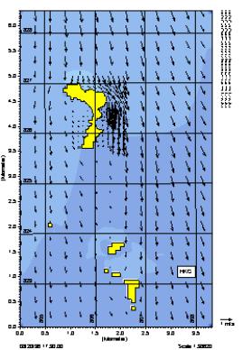
Figure 6.8 75 m model results for wet season.
Embedded 25 m and 8.3 m net.
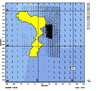
Figure 6.9 Close-up on 75 m net with embedded
25 m net and 8.3 m nets shown.
In Figure
6.10 through Figure
6.12 the calculated results for current speed, current
directions and salinity are shown for the wet season simulations as compared to
results calculated under the Pillar Point study. It is observed that good
agreement is obtained.
Figure 6.10 Comparison between previous calculated current speed and
presently calculated speeds in point (36,57) in the 75 m resolution.
Values from layer 1 (bottom) and layer 10 (surface) are shown during 5 days of
wet season simulation.
Figure 6.11 Comparison between previous calculated
current directions and presently calculated directions in point (36,57) in the
75 m resolution. Values from layer 1 (bottom) and layer 10 (surface) are
shown during 5 days of wet season simulation.
Figure 6.12 Comparison between previous calculated
current directions and presently calculated directions in point (36,57) in the
75 m resolution. Values from layer 1 (bottom) and layer 10 (surface) are
shown during entire wet season
simulation.
Based on these results for dry and wet
season simulations, it is concluded that the model adequately describes the
current conditions in the Lung Kwu Chau area.
6.2
Influence of the jetty
Based on the hydrodynamic simulations for
the dry season period with the
75 m - 25 m - 8.3 m analyses of the
influence of the jetty and the effects of the culverts have been performed. The
presence of a jetty will block a part of the north-south going water flow in
the vicinity of the coast.
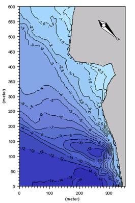
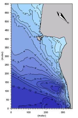
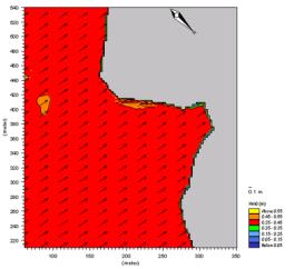
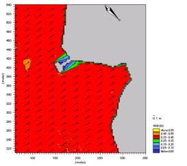
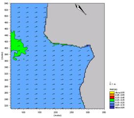
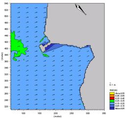
In Figure 6.13 and Figure
6.14 snapshots of the current fields without and with the
jetty during falling and rising tide are given. In Figure 6.15 difference current plots calculated as jetty scenario
minus reference scenario are given. The plots demonstrate the blocking effect
of the jetty. In the difference plots it is observed that a current difference
in the order of 0.5-1.0 m/s is present in the area around the jetty
periodically during spring tide conditions.
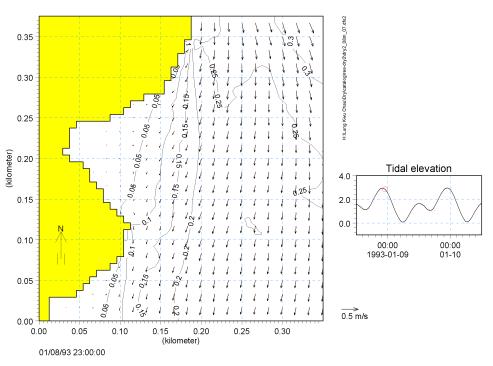
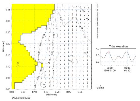
Figure 6.13 Instantaneous current plots for the
reference scenario (upper) and jetty scenario (lower) during a falling tide
situation. Contours show current magnitude. Notice that the two grid points
containing the culverts in the jetty scenario in the plot appear as water
points with small current velocities.

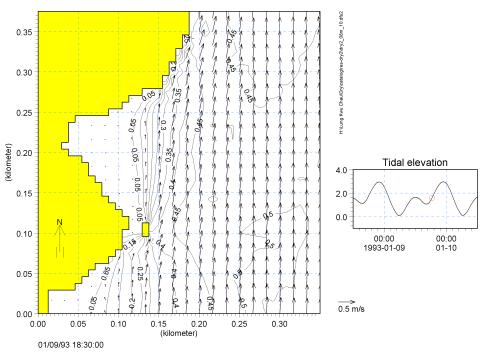
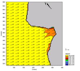
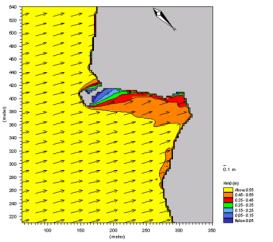
Figure 6.14 Instantaneous current plots for the
reference scenario (upper) and jetty scenario (lower) during a rising tide
situation. Contours show current magnitude. Notice that the two grid points
containing the culverts in the jetty scenario in the plot appear as water
points with small current velocities.
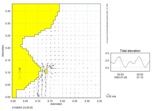
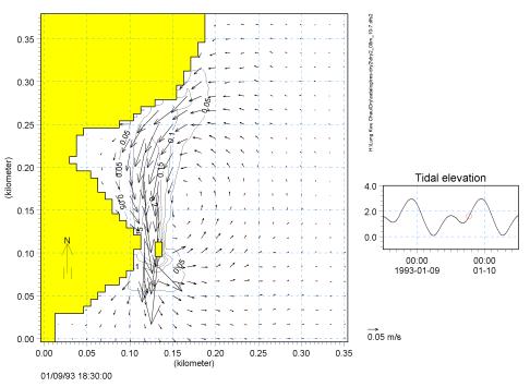
Figure 6.15 Difference current plots for falling tide
(above) and rising tide (lower) situations. Calculated as jetty scenario
current velocities minus reference scenario current velocities. Contours show
current magnitude.
6.2.1
Tracer experiment
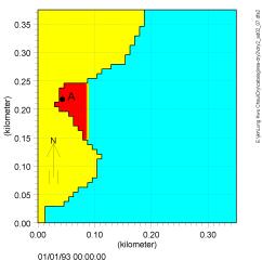
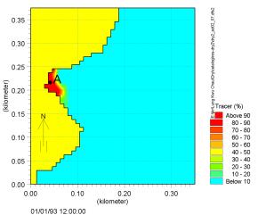
In order to assess the impact of the
proposed jetty on the flushing of the small bay north of the jetty, a numerical
tracer experiment is performed. For this purpose the advection-dispersion
module of MIKE 3 is applied. Simulations with a conservative tracer are made.
The water inside the small bay is given an initial concentration of 100,
whereas the remaining water in the model is given an initial value of 0. The
model boundary conditions are also specified as 0. In this way, the simulated
concentrations inside the small bay at any time can be interpreted as the
percentage of the initial bay water still present. Figure 6.16 shows the initial conditions of the tracer.
Figure 6.16 Initial tracer field and tracer field after
12 hours of simulation (reference scenario).
The tracer experiment was performed with
the reference scenario, with the jetty scenario and furthermore with a scenario
including the jetty and the catwalk but excluding the culverts. Figure 6.17 shows a time-series plot of tracer concentrations in
Station A (Figure 6.16). This plot shows the relatively small effect of the
jetty on the flushing of water in the small bay.
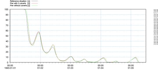
Figure 6.17 Time-series of tracer concentrations in
Station A for three different scenarios.
Culverts
The introduction of culverts in two
elements in the catwalk enables the flow to pass through the structure during
the simulation period. In Figure
6.18 the calculated flow through the culverts in the
catwalk is depicted. It is observed that the flow is of limited magnitude,
which is to be expected, since the flow is driven by the gradient in the water
level from one side of the jetty to the other.
Figure 6.18 Calculated flow discharge through culverts
in the catwalk.
6.3
Sediment spill modelling
The simulations of spreading of suspended
solids from dredging activities are performed using the PA, Particle Dispersion
model. The PA model is an add-on module to the hydrodynamic module and
simulates spreading, sedimentation and re-suspension of particulate matter
based on a pre-calculated flow field. A detailed description of the PA model background
is provided in the Methodology Report, Ref. /11/.
In order to enable a detailed 3D
description of the hydrodynamics for the sediment spreading, the nested
75 m - 25 m - 8.3 m model grid is applied.
All boundary conditions for the 75 m model are obtained from the
225 m model.
The spreading of the suspended sediment
released from the dredging works is calculated based on the proposed work
procedure and resulting expected spill.
6.3.1
Construction phase scenario
The dredging will be undertaken using one
closed grab dredger of small capacity. 5.550 m3 material is assumed
to be dredged at the site. Two scenarios are considered:
1. An
unmitigated scenario
2. A mitigated
scenario, during which silt curtains are applied.
The dredging rate for the unmitigated case
is 250 m3/day and a spill of 20kg/m3 removed mud is
expected. This amount to an average spill rate at 0.13 kg/s, based on maximum
daily rate of dredging (and assuming 11-hour working day). The dredging rate
for the mitigated case is 500 m3/day and a spill of rate of 0.065
kg/s is anticipated, based on maximum daily rate of dredging, and assuming
11-hour working day. The implementation
of silt curtains around the closed grab dredger will reduce the release of sediment
by a factor of 4 (Contaminated Spoil Management Study). Due to a doubling of the dredging rate, the
dredging sequence will only last half the period, i.e. 12 days.
The
construction phase scenarios are consequently:
· Unmitigated spill release of 0.13 kg/s during 11 hours a day for 22
days
· Mitigated spill release of 0.065 kg/s during 11 hours for 11 days
The simulations are conducted for the dry
season period.
The location of the dredging area is
shown in Figure 6.19.
The resulting output of the simulation is
the calculated time dependent excess concentrations of sediment in suspension
and areal coverage of the plume and sedimentation.
The stated
Water Quality Objectives, WQO, in the North Western Water Control Zone for
suspended solids is to remain below natural ambient level +30% and activities
may not cause the accumulation of suspended solids, which may adversely affect
aquatic communities. This criterion corresponds in this context to a surplus concentration
of 5.5 mg/l, see later in Section 7.
The sediment
is expected to be fine mud. One sample
of the seabed has been analysed for grain size distribution, and the resulting
distribution curve is shown in Drawing
3. The analysis reveal that more than 50% of the sea
bed material has a grain diameter less than 4 micron. And more than 80% of the
material has a grain diameter less than 20 micron. To represent the material,
the mean grain diameter of the material is set to 8 micron in the simulations
to include flocculation effects, and the controlling parameter in the
simulation, which is the fall velocity, is set accordingly. The fall velocity
has been determined by use of Stokes law.
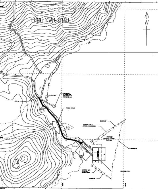
Figure 6.19 Position of the new jetty and area of
dredging.
Table 6.1 Parameters used for spreading
simulation.
|
Mean grain size diameter (micron)
|
8
|
|
Fall velocity (mm/s)
|
0.04
|
|
Shields parameter
|
0.045
|
|
Density (kg/m3)
|
2.65
|
6.3.2
Spreading simulation results
Main results from the simulation of
dredging spill are depicted in the following figures. Further results are also
presented in Section 7 on environmental impact.
For the unmitigated scenario, Figure 6.20 shows the calculated statistical maximum values of
suspended sediment concentrations based on a 24-day simulation period. The
concentration level signifies the maximum level attained at any point during
the entire period, and does consequently not represent an instantaneous
concentration level at any time.
The figure shows that generally the
highest levels of concentration in the sediment plume remain relatively close
to the island. The corresponding
results for the mitigated 11-day dredging scenario is shown in Figure 6.21.
Figure
6.22 and Figure
6.23 show the calculated sedimentation rate during the
entire simulation period. The figures also indicate which area is subjected to
increased concentration levels from the dredging spill. It is observed that
while the area to the north of the island is subjected to increased SS
concentration over a larger area, the increase is very marginal.
In comparison, Figure 6.24 and Figure
6.25 show that, as expected, the main part of the
sedimentation remains close to the island and is located south of the dredging
area. And while the northern area is subjected to sedimentation over a larger
area, the area just to the south of the location of dredging is subjected to
increased levels of sedimentation relative to the area north of the location of
dredging.
The total net sedimentation after the
simulation period is depicted in Figure
6.26 and Figure
6.27. The figures show that a thin plume propagates to the
southern model domain, but since the resulting sedimentation is very low, so is
the concentration.
Figure 6.20 Unmitigated scenario: Calculated statistical maximum values of
concentration based on a 24-day simulation period. The concentration level
signifies the maximum level attained at any point during the entire period, and
does not represent an instantaneous concentration level at any time.
Figure 6.21 Mitigated scenario: Calculated statistical
maximum values of concentration based on a 12-day simulation period. The
concentration level signifies the maximum level attained at any point during
the entire period, and does not represent an instantaneous concentration level
at any time.
Figure 6.22 Unmitigated scenario: Calculated
average sedimentation rate in kg/m2/day during the entire simulation
period.
Figure 6.23 Mitigated scenario: Calculated average
sedimentation rate in kg/m2/day during the entire simulation period.
Figure 6.24 Unmitigated scenario: Calculated average
sedimentation rate in kg/m2/day during the entire simulation period
along eastern coastline of Lung Kwu Chau.
Figure 6.25 Mitigated scenario: Calculated average
sedimentation rate in kg/m2/day during the entire simulation period
along eastern coastline of Lung Kwu Chau.
Figure 6.26 Unmitigated scenario: Total net
sedimentation in kg/m2 resulting from entire dredging sequence
during a period of 24 days.
Figure 6.27 Mitigated scenario: Total net sedimentation
in kg/m2 resulting from entire dredging sequence during a period of
12 days.
7.1
Water Quality
The
main impact of the project on the water quality around Lung Kwu Chau is
anticipated to be an increased turbidity during dredging of the seabed caused
by the release and dispersal of sediments. On this background, the following
assessment will focus on the potential impacts of the sediment dispersal on
sensitive species and habitats.
7.2
Background Conditions
The
water around Lung Kwu Chau is generally rather turbid (unclear). A high turbidity
is very common in river estuaries due to river discharges of suspended
sediment. The results of the monitoring of suspended solids at four stations in
the Sha Chau and Lung Kwu Chau Marine Park during 1997-2000 are summarised in Table 7.1. The monitoring shows depth-averaged mean
concentrations of suspended solids of 11.5 – 13.4 mg/l. The measured
concentrations ranged from 2 to 113 mg/l and even the station with lowest
maximum was 35 mg/l.
Table 7.1 Concentrations of depth-averaged
suspended solids for monitoring stations in Sha Chau and Lung Kwu Chau Marine
Park.
|
Parameter
|
Monitoring Station
|
Overall
average
|
|
SS (mg/l)
|
N Lung
Kwu Chau
|
N Sha Chau
|
SE Sha Chau
|
Pak Chau
|
|
Mean
|
13.0
|
11.5
|
12.1
|
13.4
|
|
|
Range
|
3.0 – 113.0
|
2.0 – 36.0
|
3.0 – 35.0
|
3.0 – 39.9
|
|
|
90th
percentile (ambient level)
|
20.4
|
16.0
|
17.1
|
19.5
|
18.23
|
|
30%
increase of ambient level
|
|
|
|
|
5.5
|
Data
source: AFCD routine water quality
monitoring programme for Marine Parks for period 1997 to 2000.
The
water quality objectives for marine waters in the North Western Water Control
Zone in Hong Kong, concerning the concentration of suspended solids, are the
following: "Waste discharge not to
raise the natural ambient level by more than 30%, nor cause the accumulation of
suspended solids which may adversely affect aquatic communities."
In
the assessment below, the ambient level of the concentration of suspended
solids is defined as the 90th percentile of the observations in
1997-2000. These values range from 16.0 to 20.4 mg/l at the four
stations with an average of 18.23 mg/l (Table
7.1). A 30% increase of the ambient level is thus defined
as an increase of 5.5 mg/l.
7.3
Release and Dispersal of Sediments
The
major activities involved during the construction stage of the project are
dredging for approach channel and foundation of the jetty and catwalk, filling
rubble foundations, setting precast concrete blocks, placing bermstones,
general concrete work and demolition of existing jetty. Of these activities,
only the dredging is believed to cause significant release of sediments.
The
expected amounts of sediment spill during dredging and the patterns of
dispersal and the resulting increase in concentration of suspended solids are
assessed in Section 6.3 by means of model calculations. Two scenarios have
been described. One scenario deals with unmitigated dredging and the other
considers dredging with the case that the sediment dispersal is mitigated by
means of silt curtains and shortening of the dredging period. The assumptions
of the model calculations are described above.
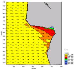
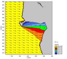
Figure 7.1 and Figure
7.2 show examples of the calculated instantaneous
concentration of suspended sediment from unmitigated dredging during southgoing
and northgoing current, respectively. During dredging, sediment plumes being
generally less than 200 m wide will go along the coast of Lung Kwu Chau.
Calculated statistical maximum concentrations above 50 mg/l and 20 mg/l,
respectively, will be experienced up to 100 and 250 m away from the working
area in case of northgoing current and at shorter distances during southgoing
current (Figure 7.5). The maximum surplus concentration is predicted to be
higher than 5.5 mg/l in the nearby bays
and just outside these in areas extending up to 400 m from the coast. However,
in the main part of these areas, SS concentrations of higher than 5.5mg/l would
occur less than 10% of the time during the 24-day simulation period (Figure 7.7).
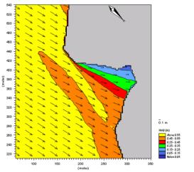
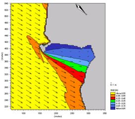
Figure 7.3 and Figure
7.4 show the calculated instantaneous concentration of
suspended sediment from mitigated dredging during northgoing and southgoing
current, respectively. During mitigated dredging, the sediment plumes will be
very narrow (20-60 m) and even in the plume, the concentrations of suspended
matter will, in general, be only slightly elevated (1-4 mg/l).
Maximum
concentrations above 20 mg/l and 10 mg/l, respectively, will be experienced up
to 200 m and 400 m away from the working area in case of northgoing
current and at shorter distances during southgoing current. The maximum surplus
SS concentration is predicted to be higher than 5.5 mg/l in an area along the
eastern coast being approximately 400m long. However, in the major part of this
area, the surplus SS concentrations would occur less than 1% of the time during
the 12-day dredging period (Figure
7.8). Even very close to the working area, elevations in
SS concentrations of higher than 5.5mg/l would occur less than 10% of the time
(less than 1 day).
From
the considerations above, even if no mitigation measures are applied, the
impact of dredging on the concentration of suspended solids will occur only on
a very local scale and through a rather short time. Furthermore, the sediment load outside the working area and very
close to this will be well below natural maximum concentrations measured in the
area during 1997 – 2000. If the impacts
of dredging are mitigated by using silt curtains and by shortening the dredging
period, the impacts on water quality will be of an even more local and
transient nature.
Figure 7.1 Calculated instantaneous concentration of
suspended solids released from unmitigated dredging for the proposed jetty at
Lung Kwu Chau during northgoing current.
Figure 7.2 Calculated instantaneous concentration of
suspended solids released from unmitigated dredging for the proposed jetty at
Lung Kwu Chau during southgoing current.
Figure 7.3 Calculated instantaneous concentration of
suspended solids released from mitigated dredging for the proposed jetty at
Lung Kwu Chau during northgoing current.
Figure 7.4 Calculated instantaneous concentration of
suspended solids released from mitigated dredging for the proposed jetty at
Lung Kwu Chau during southgoing current.
Figure 7.5 Calculated statistical maximum
concentration of suspended solids released from unmitigated dredging for the
proposed jetty at Lung Kwu Chau.
Figure
7.6 Calculated statistical maximum concentration of suspended
solids released from mitigated dredging for the proposed jetty at Lung Kwu
Chau.
Sedi. Conc > 5.5 [mg/l] in %-time
|
|
Figure 7.7 Areas in which SS
concentrations higher than 5.5 mg/l occur a certain percentage of the time
during the 24-day simulation period of unmitigated dredging for the proposed
Jetty at Lung Kwu Chau.
Sedi. Conc > 5.5 [mg/l] in %-time
|
|
Figure 7.8 Areas in which SS
concentrations higher than 5.5 mg/l occur a certain percentage of the time
during the 12-day simulation period of mitigated dredging for the proposed
Jetty at Lung Kwu Chau.
7.4
Chinese White Dolphin
The
construction of the jetty will take place in the Sha Chau and Lung Kwu Chau
Marine Park, which were established mainly to protect the population of Chinese
White Dolphin in Hong Kong Waters.
Chinese
White Dolphin is the local name of the species more broadly known as
Indo-Pacific Humpback Dolphin, Sousa
chinensis. The species are distributed throughout shallow coastal waters of
the Indian and the western Pacific Oceans, from South Africa in the west to the
northern Australia and southern China in the east (Ref. /4/).
The
Dolphins that inhabit Hong Kong waters belong to a population centred around
the mouth of Pearl River. The dolphins are distributed in the eastern Pearl
River Estuary, from the western waters of Hong Kong to at least the Zhuhai and
Macau areas. The dolphins are protected in Hong Kong by the Wild Animals
Protection ordinance, Cap. 170 (Ref. /4/)
Within
Hong Kong waters, dolphins occur only regularly to the north and west of Lantau
Island. There are seasonal changes in the distribution patterns of dolphins in
the north Lantau area. In winter and spring, dolphins are mostly seen west of
Brothers' Islands, while in summer and autumn they are more continuously
distributed in the entire North Lantau area (Refs. /5/ and /7/). This means that
dolphins explore the areas around Lung Kwu Chau throughout the year.
The
abundance of dolphins in Hong Kong waters are observed to range from 88
dolphins in spring to 145 in the summer. The best available estimate of the
total population in the Pearl River Estuary is 1028 dolphins (Ref. /4/).
The
highest abundance and widest distribution of the dolphins in Hong Kong waters
are associated with the season of the largest freshwater discharge from Pearl
River. The dolphins feed almost entirely on fish. It is believed that a high
abundance of fish associated with the mixing zone of fresh water and seawater
is a main factor determining the seasonal variations in dolphin abundance and
distribution (Refs. /4/ and /5/).
In
its entire area of distribution, the Indo-Pacific Humpback Dolphin is mainly
found in shallow coastal areas and it generally has a preference of estuarine
waters. The species in general are therefore naturally adapted to a turbid
environment. Turbidity is believed to be of minor importance for the species
itself, as the dolphins generally rely more on echolocation than on vision for
navigation and location of prey items. This also holds through for the dolphins
in the Sha Chau and Lung Kwu Chau Marine Park and in the whole North Lantau
area. These dolphins are in fact most abundant in the seasons associated with
highest natural concentrations of suspended solids.
Considering
the limited magnitude and the local nature of the impact from the dredging
operations on turbidity as well as the large area in which the dolphins are
distributed, the dolphins will hardly experience the turbidity regime during
the construction to deviate substantially for the natural conditions. However,
it cannot be totally excluded that transient and local displacements will occur
due to changes in fish distribution caused by fish avoidance of the sediment
plumes from the dredging.
The
dolphins in Hong Kong Waters are believed to be under great pressure, and
concern about the future existence of the species in Hong Kong have been
expressed (see e.g. Ref. /6/). The potential threats to the dolphins include
habitat loss caused by extensive coastal development and reclamation, intense
boat traffic causing disturbance and collisions, incidental entanglement in
fishing gear, overfishing of prey species and pollution with e.g.
organoclorides such as PCB's and DDT.
Compared
to these general threats the limited impact of the jetty construction on the
water quality around Lung Kwu Chau must be regarded as negligible, even
considering the general pressure on the dolphin population.
7.5
Impact on Benthic Organisms and
Artificial Reefs
Potential
impacts of the release of suspended sediments on benthic organisms include, in
general, shading of macroalgae (seaweeds), seagrass and stony corals, which all
depend on light for growth and survival. Furthermore, large concentrations of
suspended solids may smother the feeding organs or in other ways impair the
feeding of organisms that filter microscopic food from the water column (filter
feeders, e.g. bivalves). Furthermore, sedimentation of spilled sediments may
potentially cover and smother benthic fauna and vegetation and the settling and
establishment of the young stages of benthic fauna (larvae) and macroalgae
(spores) on the seabed may be impaired.
However,
in the present case it is important to note that all benthic species living in
the Lung Kwu Chau area must be adapted to an environment, which is generally
turbid and where very high concentrations of suspended solids occur
occasionally. Therefore, no benthic communities that are really sensitive to
increased turbidity such as coral reefs have developed in the area. As the
turbidity during dredging is not expected to deviate substantially from the
natural conditions, no impact of increased turbidity on benthic communities is
expected outside the working area and very close to this.
Along
the main part of the eastern coast of Lung Kwu Chau, the sedimentation due to
unmitigated dredging will be below 50 g/m2/day or approximately 1200
g/m2 through the whole construction period, assuming 24 days of
dredging. This corresponds to a sediment layer of 1-2 mm. The maximum
sedimentation rates in small areas near the jetty are expected to be up to 150
g/m2/day or 3600 g/m2 through the whole construction period,
corresponding to a sediment layer of 3-4 mm. In most of the impacted area, the
sedimentation induced by mitigated dredging will be below 100 g/m2
through the whole period, corresponding to a sediment layer of 0.1 mm. Only in
very small areas, the total sedimentation will exceed 500 g/m2
corresponding to a layer of approximately 0.5 mm. The impact of
dredging-induced sedimentation on Gorgonian soft corals, that have been
observed on a shipwreck off the coast approximately 200-300 m north of the
working area, is therefore predicted to be minimal. As the natural seabed in the bay areas consists mainly of soft
sediments (sand and mud), even the local impact of sedimentation on benthic
organisms are expected to be limited and temporal of nature.
An
artificial reef has been established in the Marine Park about 2 km south of
Lung Kwu Chau. A biological community will develop or have already developed on
this artificial reef. No description of the biological colonisation of the
artificial reef has been available for the present assessment. However, the
community is likely to be made up of sessile animal species like soft corals,
sponges, barnacles, bivalves, squirts (tunnicates), bryozoans and an associated
mobile fauna of crustaceans, sea stars, brittlestars and fish. Some seaweed
species may also colonise the artificial reef, if the light conditions allow
for this. However, as was the case for the fauna in the area in general, only
species adapted to a rather high turbidity will colonise the artificial reef. Furthermore,
the model calculations show that the artificial reef will be virtually
unaffected by sediment from the dredging operations (Figure 7.9 and Figure
7.10). Therefore, no impact of the jetty construction on
the marine life on the artificial reef is expected. The same conclusion is
judged to be valid for the occurrences of Gorgonian soft corals that have been
observed at some locations near Tree Island and Sha Chau.
7.6
Other Impacts on Water Quality
Other
potential impacts of the project on the water quality include the release of
inorganic nutrients from the dredged sediments, giving rise to an increased
growth of phytoplankton. Similar organic and inorganic oxygen consuming
substances may be released leading to local decreases in water oxygen content.
However, due to the limited sediment release and the short duration of the
work, these impacts are expected to be negligible and the water quality
objectives concerning these parameters (Table
7.2) are expected not to be violated.
The
presence of the proposed jetty and catwalk may cause some degree of
interference with the existing water circulation pattern, which again may lead
to changes of the water quality. However, simulation results reveal that no
major interception of water current is to be expected. Thus, the permanent
impact of the project on the water quality around Lung Kwu Chau is anticipated
to be small and to occur only on a very local scale.
Figure 7.9 Location of the
artificial reef and the calculated statistical maximum concentrations of
suspended sediments from unmitigated dredging for the jetty at Lung Kwu Chau.
Figure 7.10 Location of the artificial reef and the
calculated sedimentation rates during unmitigated dredging for the jetty at
Lung Kwu Chau.
Table 7.2 Summary Statistics (mean and range) of
Water Quality of Sha Chau and Lung Kwu Chau Marine Park in 1997 – 2000.
|
Parameter
|
|
Monitoring Station
|
WPCO WQOs (in marine
waters)
|
|
|
|
|
|
SE Sha Chau
|
Pak Chau
|
|
|
Temperature (oC)
|
|
24.0
(10.0
– 30.3)
|
24.1
(10.0
– 30.0)
|
24.2
(10.0
– 34.0)
|
24.2
(10.0
– 31.0)
|
natural
daily level
± 2 oC
|
|
Salinity (ppt)
|
|
26.5
(3.0
– 36.9)
|
26.4
(3.0
– 36.2)
|
26.7
(3.0
– 36.2)
|
26.3
(2.5
– 36.9)
|
natural
ambient level
± 10 %
|
|
DO (mg L-1)
|
Surface
|
6.9
(4.4
– 8.5)
|
6.9
(4.4
– 9.0)
|
6.9
(4.6
– 8.9)
|
6.9
(4.4
– 8.8)
|
³ 4 mg L-1
|
|
|
Bottom
|
5.6
(1.9
– 8.6)
|
6.0
(3.5
– 9.0)
|
6.1
(3.1
– 8.7)
|
6.0
(2.4
– 8.9)
|
³ 2 mg L-1
|
|
pH value
|
|
8.1
(7.6
– 8.4)
|
8.1
(7.6
– 8.4)
|
8.1
(7.7
– 8.4)
|
8.1
(6.7
– 8.3)
|
6.5
- 8.5 (± 0.2 from natural range)
|
|
Turbidity (NTU)
|
|
15.6
(1.0
– 146.0)
|
9.67
(0.5
– 42.1)
|
13.22
(0.7
– 85.0)
|
11.8
(0.85
– 44.0)
|
-
|
|
SS (mg L-1)
|
|
13.0
(3.0
– 113.0)
|
11.5
(2.0
– 36.0)
|
12.1
(3.0
– 35.0)
|
13.4
(3.0
– 39.9)
|
£ natural ambient level
+30%
|
|
BOD5
(mg L-1)
|
|
0.80
(0.01
– 2.27)
|
0.80
(0.05 – 1.99)
|
0.80
(0.04
–2.31)
|
0.83
(0.14
–2.14)
|
not
applicable to
marine
waters
|
|
Ammoniacal Nitrogen
(mg L-1)*
|
|
0.17
(0.02
– 0.64)
|
0.17
(0.01
– 0.76)
|
0.17
(0.02
– 0.76)
|
0.16
(0.03
– 0.72)
|
-
|
|
Total Inorganic Nitrogen
(mg L-1)*
|
|
1.56
(0.03
– 8.29)
|
1.61
(0.04
– 8.87)
|
1.56
(0.04
– 7.68)
|
1.61
(0.04
– 8.87)
|
£ 0.5 mg L-1
|
|
Total Phosphorus (mg L-1)*
|
|
0.10
(<0.02
– 0.31)
|
0.10
(<0.02
– 0.62)
|
0.08
(<0.02
– 0.35)
|
0.10
(<0.02
– 0.65)
|
-
|
|
Chlorophyll-a
(µg L-1)
|
|
2.94
(0.21
– 16.3)
|
2.8
(0.5
– 22.4)
|
6.5
(0.3
– 16.0)
|
2.6
(0.5
– 19.7)
|
-
|
|
Unionized Ammonia
(mg L-1)**
|
|
0.04
(0.01
– 0.09)
|
0.04
(0.0
– 0.09)
|
0.04
(0.01
– 0.11)
|
0.04
(0.01
– 0.11)
|
£ 0.021 mg L-1
|
|
E.coli (colonies/ 100ml)**
|
|
90.2
(0.0
– >200)
|
63.5
(0.0
– >200)
|
65.4
(0.0
– >200)
|
39.4
(0.0
– 97.5)
|
|
Notes:
1 The presented data are depth-averaged
data, except when specified otherwise
2 * = Average between 1998-2000.
3 ** = Data for year 2000
This
section describes the methodology and data used in the assessment of the impact
that construction of the projected jetty at Lung Kwu Chau may have on beach morphology,
together with the results obtained and the conclusions reached.
8.1
Description of Problem
There
is some concern that construction of the projected jetty at Lung Kwu Chau may
have a negative impact on the morphology of the beach located immediately to
the north of the rocky headland where the jetty will be constructed. The
position of the jetty and the beach are indicated on Figure 8.1 below.
Position of projected jetty
|
|


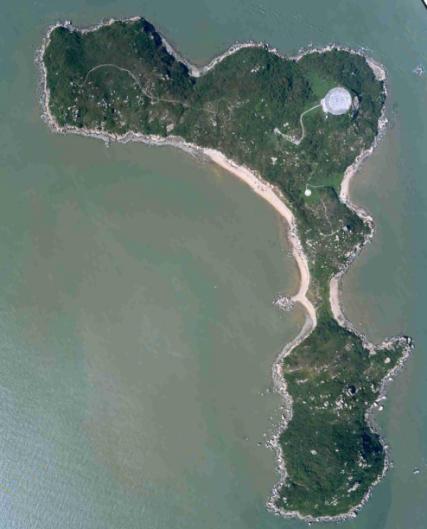
Figure 8.1 Aerial photograph of Lung Kwu Chau, where
the position of the projected jetty and the beach subject of the present
assessment have been indicated
Figure 8.1 shows that the beach is a small pocket beach that
extends between two rocky headlands, which keep the beach in place. Figure 8.2 and Figure
8.3 show a view from the sea of the beach and of the
existing jetty.
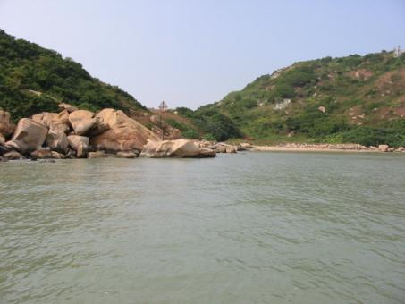
Figure 8.2 View of the beach from the sea
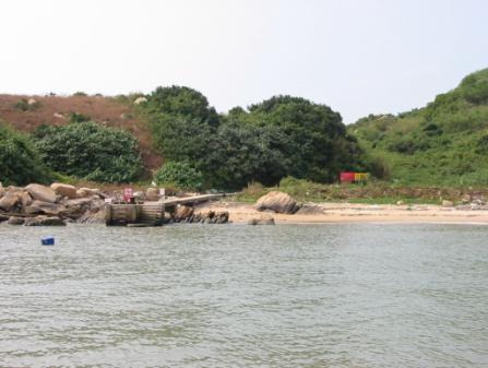
Figure 8.3 The beach and the existing jetty seen
from the sea
Construction
of the planned jetty could impact on the beach morphology if the shadow zone
that the new jetty will generate on its lee side encompasses the beach.
Accumulation of sediment in the lee side of shore-normal structures such as
groins and jetties due to the current that flows towards the area protected
from the incident waves by the structure is a well-known mechanism in coastal
engineering practice. The morphological impact assessment that is described in
further detail in the following sections of this note has been based on this
concept.
8.2
Study Methodology
The
east coast of Lung Kwu Chau is well protected from waves from westerly directions
due to its location close to Hong Kong peninsula and Lantau Island, see Figure 8.4.

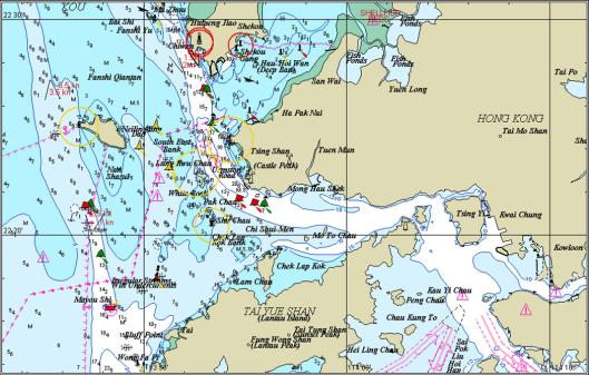
Figure 8.4 Sea chart showing location of Lung Kwu
Chau relative to Hong Kong and Lantau. ã C-Map, Norway
Waves
reaching the eastern coast of Lung Kwu Chau are therefore locally generated by
winds blowing from easterly directions and possibly also from north and south.
Based
on the above discussion and on the approach described in Section 8.1, the morphological impact assessment has consisted of
the following tasks:
1.
Establishment of yearly-averaged
wind-wave climate off Lung Kwu Chau
2.
Detailed analysis of wave conditions
in the vicinity of the project site, both for the present situation and after
construction of the jetty and dredging of the approach channel
3.
Assessment of impact on beach
morphology based on the comparison of the results obtained from the propagation
of selected wave cases for the existing conditions and after construction of
the jetty
Tasks
1 and 2 are described in further detail in the following sub-sections, while
the analysis of results and assessment of impact on beach morphology are
discussed in Section 3 of the present note.
8.2.1
Yearly mean wind-wave climate off the
eastern coast of Lung Kwu Chau
DHI's
nearshore wind-wave model MIKE 21 NSW was used to generate the yearly mean
wind-wave climate off the eastern coast of the island.
MIKE
21 NSW MIKE 21 NSW is a spectral wind-wave model, which describes the
propagation, growth and decay of short-period waves in nearshore areas. The
model includes the effects of refraction and shoaling due to varying depth,
wave generation due to wind and energy dissipation due to bottom friction and
wave breaking. The effects of current on these phenomena are included. For
additional details regarding MIKE 21 NSW, cf. Ref. /8/ and the User Guide for
the model.
Wind
statistics derived from 12 years of wind records at Lau Fau Shan automatic
weather station, Ref. /9/, were used as input for the generation of wind-waves
using the MIKE 21 NSW model. Wind data are presented in tabular form, as
percentage frequency of occurrence of hourly wind direction and speed, at 30°
intervals for wind direction and for wind speed classes 0-3.2 m/s,
3.3-8.2 m/s, 8.3-14.2 m/s and >14.2 m/s. Very few data fall in the last wind speed
class, thus indicating that wind conditions in the area are relatively mild.
The wind rose corresponding to the data used in
the present study is shown in Figure
8.5 below.
Figure 8.5 Wind rose for Lau Fau Shan (1986-1997)
The figure shows that
prevailing winds in the area are from the NE-SE sector.
Model
bathymetries were generated using information about the variation of water
depths in the area available from digital sea charts. Due to MIKE 21 NSW
requirement regarding the maximum allowable angle between wind (wave) direction
and the x-axis of the model bathymetry (which points towards land), a number of
bathymetries were generated to accommodate all winds between north and south,
i.e. wind directions between 0° and 180°. The bathymetry used to generate wind-waves corresponding to wind
from east is shown as an example in Figure
8.6. Note that north is pointing downwards in this
figure.

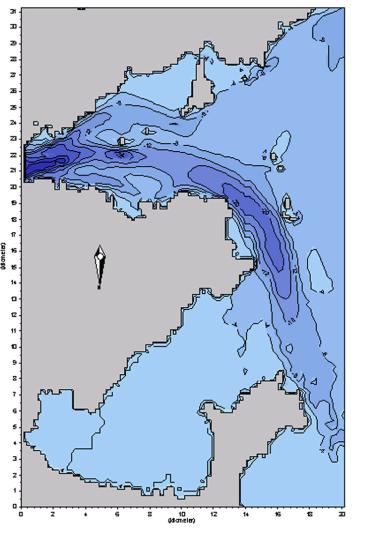
Figure 8.6 MIKE 21 NSW model bathymetry
As
Figure 8.6 shows, the water depths in the area around Lung Kwu Chau
range between 4 m and 8 m. A shallow area around continental Hong
Kong, with depths less than 4 m can also be seen. A deep channel (Urmston
Road) separates Lung Kwu Chau from the mainland.
The
wave rose corresponding to the yearly mean wind-wave climate generated using
MIKE 21 NSW off Lung Kwu Chau is shown in Figure
8.7.
Figure 8.7 Wave rose for wind-waves off the eastern
coast of Lung Kwu Chau generated by MIKE 21 NSW
Analysis
of Figure 8.7 leads to the following conclusions:
·
Almost 50% of the time, the
significant wave height Hm0 is less than 0.05 m
·
Waves off the eastern coast of the
island have a significant wave height predominantly between 0.05 m and
0.30 m
·
No waves approach the island from
directions 30° and 60°. This is due to the presence of the deep channel (Urmston Road)
which refracts (turns) the waves from these directions towards north. This is
the reason why waves from north seen to be over-represented in Figure 8.7 when it is compared to the wind rose in Figure 8.5.
·
Highest waves approach the island from
north and east. For waves from north, this is due to a combination of the
relatively long fetches and strong winds associated with directions 0°, 30° and 60°. For
waves from east, the high waves are due to the strong winds from this direction
and the large water depths that exist between Lung Kwu Chau and the mainland
·
The wave rose shown in Figure 8.7 is in qualitatively good agreement with the alignment
of the beach being investigated, cf. Figure
8.1. A stable beach will tend to assume an orientation
that faces the prevailing waves, in such a way that its alignment corresponds
to zero net yearly transport. As Figure
8.1 shows, the beach is aligned in such a way that its
normal is slightly turned southward with respect to due east, which agrees well
with the wave rose shown in Figure
8.7. Note that the beach is protected from waves from
north by the rocky headland and promontory on its northern side.
8.2.2
Detailed analysis of wave conditions
in the vicinity of the project site
Five
wave conditions (combination of significant wave height Hm0, peak
period Tp and mean direction of wave propagation MWD) were selected
from the nearshore yearly mean wind-wave statistics generated with MIKE 21 NSW,
cf. Figure 8.7. Since construction of the projected jetty will not
modify the wave conditions along the beach for waves propagating from north,
this direction was not taken into account in the analysis.
The
wave conditions as applied along the offshore boundary of the model bathymetry
(see Figure 8.8 for details) are listed in Table 8.1 below.
Table 8.1 Wave conditions used in the analysis
|
Wave case #
|
Hm0
(m)
|
Tp
(s)
|
MWD
(°N)
|
Type of spectrum
|
n
(-)
|
|
1
|
0.45
|
2.6
|
100
|
JONSWAP
|
5
|
|
2
|
0.60
|
2.9
|
120
|
JONSWAP
|
5
|
|
3
|
0.60
|
2.9
|
150
|
JONSWAP
|
5
|
|
4
|
0.60
|
2.9
|
170
|
JONSWAP
|
5
|
|
5
|
0.25
|
2.3
|
120
|
JONSWAP
|
5
|
If
the wave heights in Table 8.1 are compared to the wave rose in Figure 8.7, it can be seen that rather large values have been
used in the detailed analysis of wave conditions in the vicinity of the jetty.
This was done on purpose, in order for the analysis to be conservative and
therefore on the safe side.
DHI's
wave model MIKE 21 PMS was used for the analysis. MIKE 21 PMS is based on a
parabolic approximation to the elliptic mild-slope equation governing the
refraction, shoaling, diffraction and reflection of linear water waves
propagating on gently sloping bathymetry. For additional information about the
theoretical backgorund of the model, cf. Ref. /10/ or the User Guide for MIKE
21 PMS.
MIKE
21 PMS can be applied to any water depth on a gently sloping bathymetry, and it
is capable of reproducing phenomena, such as shoaling, refraction, dissipation
due to bed friction and wave breaking, forward scattering and diffraction. This
last feature is of special importance for the present study, in which
diffraction of the waves due to the presence of the jetty and the associated
currents that are generated may have a negative impact on the morphology of the
pocket beach.
An
additional feature of MIKE 21 PMS is the ability to simulate directional and
frequency spreading of the propagating waves by use of linear superposition.
This feature was used in the simulations by prescribing irregular, directional
waves at the offshore boundary of the model bathymetry, cf. Table 8.1. A relatively low value of the directional spreading
index n was used, keeping in mind
that the waves are wind-generated. n is the exponent in the directional
distribution of wave energy given by cosn|q-qm|, where qm = MWD is the mean direction of wave
propagation.
In
order to assess the impact that construction of the jetty will have for the
wave conditions along the pocket beach, two model bathymetries were generated.
The first one corresponds to the existing conditions (i.e. no jetty) while the
second bathymetry includes the projected jetty and dredging of an approach
channel to –2.5 m CD. The two bathymetries are shown in Figure 8.8. It must be noted that the bathymetries have been
rotated due to modelling requirements already discussed in Section 8.2.1.
Figure
8.8 MIKE 21 PMS model
bathymetry. Existing situation (left) and with jetty and dredging included
(right)
8.3
Results and Conclusions
The
results obtained from the propagation of wave cases #1 to #5 in Table 8.1 using MIKE 21 PMS on the two bathymetries shown in Figure 8.8 are presented in Figure
8.9 to Figure
8.13 below. Results obtained for the existing conditions
are shown to the left of each figure, whereas results including the projected
jetty are shown to the right.
Results
are presented in the form of contours of significant wave height Hm0
and vectors indicating the direction of wave propagation, with the length of
the vectors scaled according to the local wave height. The lowest level of the
colour scale (dark blue) corresponds to Hm0 < 0.05 m. The
scale has uniform increments of 0.10 m in significant wave height, meaning
that red areas correspond to 0.35 m < Hm0 < 0.45 m
and yellow areas to Hm0 > 0.55 m.
Note
that only a part of the area covered by the models has been shown in Figure 8.9 to Figure
8.13 inclusive, in order to focus attention on the
analysis of the results along the pocket beach being investigated.
Figure 8.9 Wave fields corresponding to Hm0
= 0.45 m, Tp = 2.6s and MWD = 100°N calculated with MIKE 21 PMS. Existing
situation (left) and with jetty and dredging included (right)
Figure 8.10 Wave fields corresponding to Hm0
= 0.60 m, Tp = 2.9s and MWD = 120°N calculated with MIKE 21 PMS. Existing
situation (left) and with jetty and dredging included (right)
Figure 8.11 Wave fields corresponding to Hm0
= 0.60 m, Tp = 2.9s and MWD = 150°N calculated with MIKE 21 PMS. Existing
situation (left) and with jetty and dredging included (right)
Figure 8.12 Wave fields corresponding to Hm0
= 0.60 m, Tp = 2.9s and MWD = 170°N calculated with MIKE 21 PMS. Existing
situation (left) and with jetty and dredging included (right)
Figure 8.13 Wave fields corresponding to Hm0
= 0.25 m, Tp = 2.3s and MWD = 120°N calculated with MIKE 21 PMS. Existing
situation (left) and with jetty and dredging included (right)
Analysis
of Figure 8.9 to Figure
8.13 leads to the following conclusions:
·
For waves lower than Hm0 =
0.50 m and propagating from 100°N and 120°N
(corresponding to cases #1 and #5 in Table
8.1), construction of the jetty and dredging of the
approach channel to –2.5 m CD will not change the wave conditions
along the beach compared to the present situation. This is shown by Figure 8.9 to Figure
8.13, and means that for the wave conditions prevailing in
the area (cf. Figure 8.7), construction of the jetty will not have any
negative impacts on the morphology of the beach
·
For higher waves approaching the beach
from 120°N (corresponding to case #2 in Table
8.1), construction of the jetty and dredging of the
approach channel will only change the wave conditions along the beach
marginally, as shown in Figure
8.10. Thus, it is deemed that construction of the
projected jetty will not have any negative impacts on the morphology of the
beach for these wave conditions
·
It may appear as if the differences
between the wave fields calculated with and without the jetty for wave cases #3
and #4 in Table 8.1 are more important than for the other three cases,
see Figure 8.11 and Figure
8.12. However, it is important to keep in mind that waves
are small event for the present condition, due to the sheltering effect of the
headland to the south of the beach. Another aspect to consider is that the
waves for cases #3 and #4 have limited occurrence during the year, 0.12% and
0.16%, respectively, as shown by the wave rose in Figure 8.7. Based on these two facts, it is concluded that
construction of the jetty and dredging of the access channel will not have
negative impacts on the beach morphology, even for the case of relatively high
waves from directions 150°N and 170°N.
/1/ Methodology
Report on modelling and assessment approach for Lung Kwu Chau Jetty.
DHI/Maunsell, 2002. For EPD.
/2/ SSDS
Stage II: Oceanic Outfall, Oceanographic Survey and Modelling. Report (R7a)
Tidal Flow Model, Dry Season Calibration. SOM Consultant, September 1994.
/3/ Pillar
Point Outfall Study Report. Calibration of hydrodynamic models. DHI/Unisearch
and Montgomery Watson, 2000. For EPD.
/4/ Agriculture,
Fisheries and Conservation Department. (2000). The Conservation Programme for
the Chinese White Dolphin in Hong Kong. AFCD 2000.
/5/ Jefferson,
T 1998, Population Biology of the Indo-Pacific Hump-backed Dolphin (Sousa
chinensis Osbeck, 1765) in Hong Kong Waters: Final Report, submitted to
Agriculture and fisheries Dept. Hong Kong SAR Government 15 April 1998.
/6/ Liu and
Hills 1997. Environmental Planning, Biodiversity and the Development Process:
The Case of Hong Kong's Chinese White Dolphins. Aquatic Mammals 24.3. 91-110.
/7/ Parsons,
E. C. M. 1998. The behaviour of Hong Kong's resident cetaceans: the
Indo-Pacific hump-backed dolphin and the finnless porpoise. Journal of Environmental
/8/ Holthuijsen,
L H, Booij, N & Herbers, T H C (1989): "A Prediction Model for
Stationary, Short-crested Waves in Shallow Water with Ambient Currents", Coastal Eng., 13, 23-54.
/9/ Hong Kong Observatory, Climatology of Lau Fau Shan 1986-1997 –
Technical Note No. 95, by M.C. Ng & W.M. Chan, April 1999.
/10/ Kirby, J T (1986): "Rational
Approximations in the Parabolic Equation Method for Water Waves", Coastal Eng., 10, 355-378.
/11/ Fax
message from Maunsell containing: 'Site Plan, Improvement works to Lung Kwu
Chau Jetty, Drw. No. P20278-1B'.
Drawing 1 Typical current field
(m/s) calculated in 675 m during neap period, outgoing flow during dry
season.
Drawing 2 Typical current flow
(m/s) calculated in 675 m grid during neap tide, incoming flow during dry
season.
Drawing 3 Grain size distribution curve.