C2 Modelling Details
C2.1 Introduction
The refinement of grid has been applied in the Delft-WAQ model in the EIA Study. This enhanced the resolution of the model at the sensitive receivers in the vicinity of the project area. The refined model grid mesh adopted in the EIA Study is shown in Figure C2.1. As shown, the grid size of the refined grid mesh is less than 75 m.
Figure C2.1 Refined Water Quality Model Grid used in the EIA
C2.2 Theory of the Grid Refinement
C2.2.1 Mass Conserving Properties of the Refinement
The refinement of the water quality grid is carried out at the level of the finite volumes used by the computational core of the Delft3D-WAQ programme. The text below assumes that the model is 3D. The finite water volume is given by V(t), while there are 6 flows Q(t) through the surfaces of the finite volume (see Figure C2.2). Note that in the surface and the bottom layer one of the two vertical flows is zero by definition.
Figure 2.2 Definition of the Water Balance of a Finite Volume
The water balance of the finite volume is defined as follows:
![]()
The demonstration of mass conservancy for the refinement of the grid is based on the assumption that the mass balance for one finite volume (expressed by the equation above) is valid.
The refinement is carried out in the horizontal plane only (in the x and y directions). In x-direction the finite volume is sliced in M parts (M ³ 1), and in the y-direction the volume is sliced in N parts (N ³ 1).
We assume that the bottom surfaces as well as the top surfaces are plane: this implies that the bottom depth and the water level within one vertical column of finite volumes are assumed constant.
First, we present the water balance terms of one of the sub-volumes. Next we will demonstrate that the conservancy of mass for the whole volume implies the conservancy of mass for each of the subvolumes. The subvolumes are indicated by indices:
i, i = 1,M
j, j = 1,N
Each of the sub-volumes (i,j) is given an equal share of the total volume:
![]()
In a similar way the vertical flows are simply divided homogeneously over each of the N x M sub-volumes:

The horizontal flows are first interpolated from one side to the other side of the total volume, and afterwards sliced in the necessary number of equal parts:


The water balance of one sub-volume (i,j) is defined as follows:
![]()
If we substitute all expressions above in the water balance equation for one sub-volume, it is easily demonstrated that the water balance equation for the total volume remains. Thus, if the water balance for the total finite volume is correct, also the water balance for each of the sub-volumes is correct.
C2.3 Acceptability of Unrefined FLOW Model
C2.3.1 Introduction
The results submitted to the draft EIA have been obtained by using a local grid refinement in the water quality model. This refinement technique uses the flow data from the unrefined FLOW model. The refinement (Figure C2.1) is intended to provide resolution of concentration gradients on spatial scales smaller than that of the FLOW model grid (similar results could have been obtained e.g. by a particle tracking approach).
It is recognised that the grid refinement method does not provide higher resolution flow patterns. However, in this specific case, it will show in the following section that the results submitted can be an acceptable basis for the impact assessment.
C2.3.2 Comparison between Unrefined and Refined Flow Model
From the results obtained it has been derived that the area where a significant impact from the construction or the operation of the project can possibly be expected is the area immediately adjacent to the project construction site and the Castle Peak B discharge location respectively.
A domain decomposition model was used to assess the small scale velocity variations and to compare them with the unrefined flow field calculated by the Western Harbour Model (Figure C2.3).
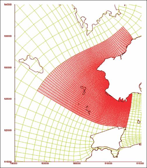
Figure C2.3 Refined Domain (red) and Unrefined Domain (green) of the DD-FLOW Model
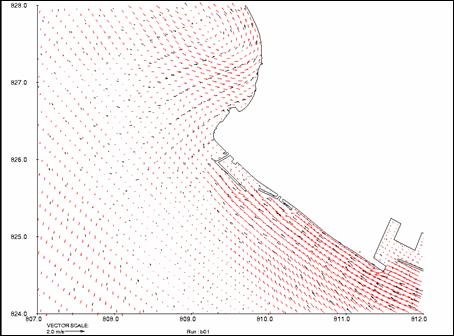
From the simulation results (wet season) available at present, we have produced velocity vector snapshots for the ebb and the flood currents near the project area (spring tide conditions); see Figures C2.4 and C2.5.
Figure
C2.4 Comparison of flood currents in the wet season calculated by the
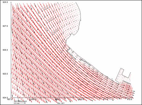
Figure
C2.5 Comparison of ebb currents in the wet season calculated by the
From the comparative velocity vector fields, it can be derived that there are no major differences between the overall features of the currents in and around the project area calculated by both models. On theoretical grounds we may assume that the unrefined model misses some smaller scale currents patterns which are resolved by the DD-FLOW model with the locally refined model.
This phenomenon is not likely to affect the dispersion of the operational discharges through outfall B of Castle Peak Power Station, since this discharge is in the area with high currents parallel to the coast.
The sediments released during the construction of the project may reach the area with smaller currents velocities north of the site. In this area, the unrefined model may underestimate the dispersion of sediments by small scale currents. This will lead to overestimated impacts close to the project site. From the most conservative perspective, this does not affect the reliability of the assessment, as long as no water quality objectives are violated in the simulation results. Farther away from the project site, e.g. at sensitive receivers B1, I5 and I3, the impacts may be underestimated. However, the impacts are well below the applicable objectives, and therefore this extra degree of uncertainty does not affect the results of the EIA.
The approach of interpolation of the flow results onto the refined water quality model has been used in recent EIA studies, among those the modelled areas in the EIA for the Permanent Aviation Fuel Facility ([1]) and the EIA for New Contaminated Mud Pits ([2]) are the adjacencies to the modelled area for this Study. Hence, it is believed that the approach is likewise suitable for this Study.