1
Methodology used for the grid refinement
The
applied grid refinements have been realised in the Delft3D-FLOW model by means
of the so-called domain decomposition technique. The FLOW model grid has subsequently
been adopted without further aggregation in the water quality models.
Domain
decomposition is a technique in which a model domain is subdivided into several
smaller model domains, which are called sub-domains. Domain decomposition allows for local
grid refinement, both in horizontal direction and in vertical direction. Grid refinement in horizontal direction
means that in one sub-domain smaller mesh sizes (fine grid) are used than in
other sub-domains (coarse grid) (see Figures
1.1 and 1.2).
The
FLOW computations are carried out separately on the sub-domains. The communication between the
sub-domains takes place along internal open boundaries, or so-called dd-boundaries.
The resulting equations are solved simultaneously for all boundaries.
In
the current model, 5 horizontally refined sub-domains are distinguished. The
division in sub-domains is based on the requirements for horizontal model
resolution in order to represent the coastline and bathymetry near the project
sites and to adequately simulate physical processes.
The
domain decomposition approach implemented in Delft3D-FLOW is based on a
subdivision of the domain into non-overlapping sub-domains. An efficient iterative method is used
for solving the discretised equations over the
sub-domains. A direct iterative
solver is used for the continuity equation, which is comparable to the single
domain implementation. For the
momentum equations, the transport equation and the turbulence equations the
so-called additive Schwarz method is used, which allows for parallelism over
the sub-domains. Upon convergence,
this type of iteration process is comparable to the corresponding iterative
solution methods in the single domain code, and features a comparable
robustness. As witnessed by
numerical experiments carried out during the development of the technique, the
differences introduced by separating domains turn out to be of insignificance.
Figure 1.1 Refinement
of Model Grid of the Model in the Vicinity of Soko Islands
Figure 1.2 Refinement
of Model Grid of the Model in the Vicinity of Black Point
The
verification of the correct implementation of the grid refinement has been
carried out by graphically comparing the results from the original, unrefined
model with the refined model. This
has been done for two locations:
·
A location near the intake point of Black
Point Power Station, inside the refined domain around the Black Point site.
·
A location northwest of South Soko Island (SR26), inside the refined domain around the South Soko site.
·
A location west of Lantau,
inside the refined domain around the Fan Lau .
The
results are shown in Figures 1.3, 1.4,
1.5 (wet season) and Figures 1.6,
1.7 & 1.8 (dry season). The comparison includes the water level
(top graph), the current speed (second graph), the surface and bottom salinity
(third graph) and the surface and bottom temperature (bottom graph). The comparison has been carried out for
both the wet and the dry season simulations.
The
results clearly demonstrate that the overall behaviour of both models is
consistent, while the results are slightly different in the details. This is exactly as it would be expected
from a locally refined model.
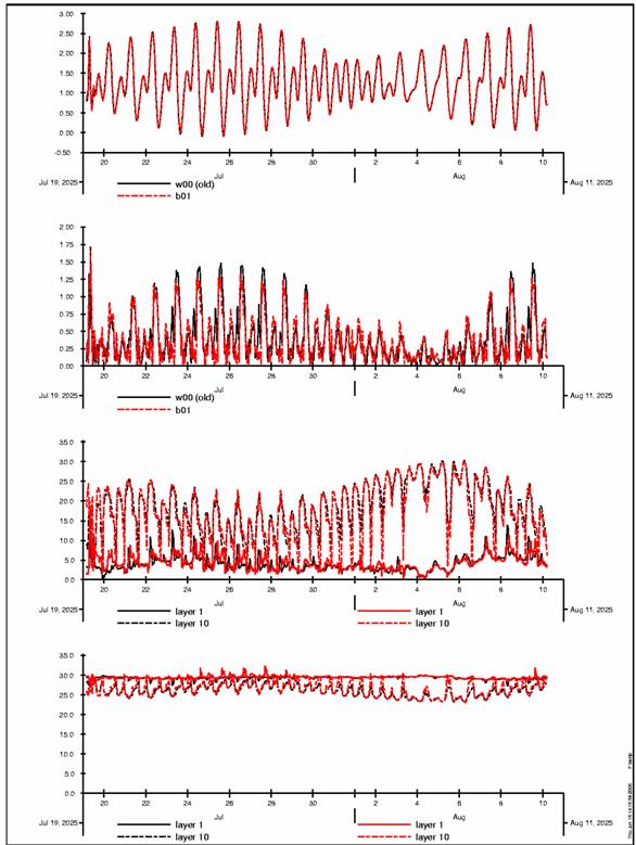
Figure 1.3 Comparison
(Wet Season) between Unrefined Model (in black) and Refined Model (in red) at
the Black Point Power Station Intake in (Top graph: Water
Level; Second graph: Current Speed; Third graph: Surface (layer 1) and Bottom
(layer 10) Salinity; and Bottom graph: Surface (layer 1) and Bottom
Temperature)
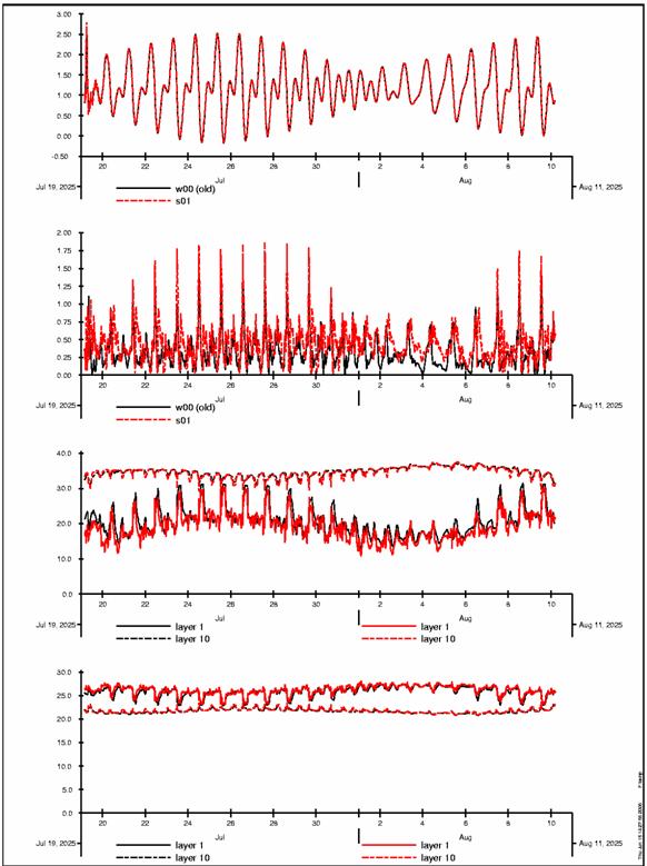
Figure 1.4 Comparison
(Wet Season) between Unrefined Model (in black) and Refined Model (in red) at North western Side of South Soko (Top graph: Water
Level; Second graph: Current Speed; Third graph: Surface (layer 1) and Bottom
(layer 10) Salinity; and Bottom graph: Surface (layer 1) and Bottom
Temperature)
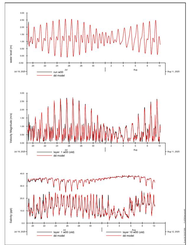
Figure 1.5 Comparison
(Wet Season) between Unrefined Model (in black) and Refined Model (in red) at West Lantau (Top
graph: Water Level; Second graph: Current Speed; and Third graph: Surface
(layer 1) and Bottom (layer 10) Salinity.
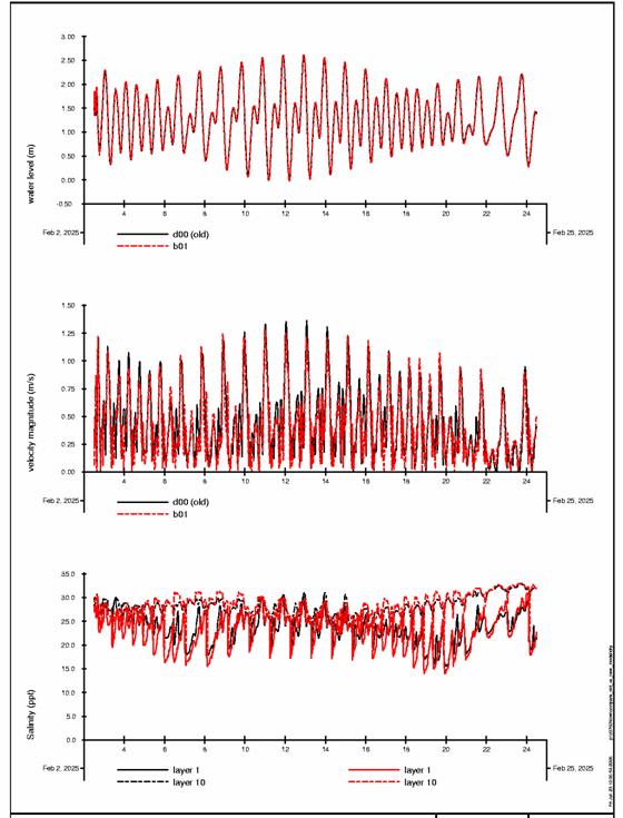
Figure 1.6 Comparison
(Dry Season) between Unrefined Model (in black) and Refined Model (in red) at
the Black Point Power Station Intake in (Top graph: Water
Level; Second graph: Current Speed; and Third graph: Surface (layer 1) and
Bottom (layer 10) Salinity.
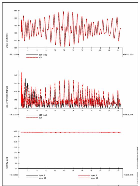
Figure 1.7 Comparison
(Dry Season) between Unrefined Model (in black) and Refined Model (in red) at
North western Side of South Soko
(Top graph: Water Level; Second graph: Current Speed; and Third graph:
Surface (layer 1) and Bottom (layer 10) Salinity.
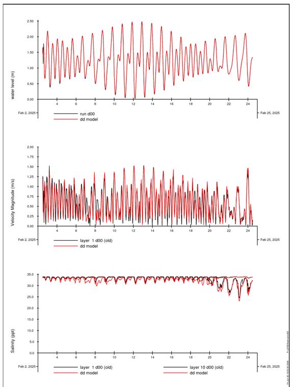
Figure 1.8 Comparison
(Dry Season) between Unrefined Model (in black) and Refined Model (in red) at West Lantau (Top
graph: Water Level; Second graph: Current Speed; and Third graph: Surface
(layer 1) and Bottom (layer 10) Salinity.
All
hydrodynamic scenarios are simulated for a spring-neap-cycle during the dry
season and a spring-neap-cycle during the wet season. The simulated periods are:
·
Dry season: simulation period from 2
February 12:00h to 22 February 12:00h, simulation period 20 days, time step 30
seconds.
·
Wet season: simulation period from 19 July
04:00h to 10 August 04:00h, simulation period 22 days, time step 30 seconds.
Adequate
spin-up has been provided for salinity and temperature by means of initial
conditions files (as shown by verification results). The first 5 days of both simulation
periods are also used as spin-up, and are not used for the assessments purpose.
The
wind has been set to typical seasonally averaged values:
·
Dry season: northeast, 5 m s-1.
·
Wet season: southwest, 5 m s-1.
The
rivers have been set to typical seasonal values:
Dry
(m3 s-1) Wet
(m3 s-1)
Humen 1248 7442
Jiaomen 527 4732
Hongqili 128 1535
Hengmen 136 2805
Deep
Bay 2.5 16